Segmented Diagnose (Classification)

Experiment initialization and data preparation

from piml import Experiment
from piml.models import XGB2Classifier

exp = Experiment()
exp.data_loader("SimuCredit", silent=True)
exp.data_summary(feature_exclude=["Race", "Gender"], silent=True)
exp.data_prepare(target="Approved", task_type="classification", silent=True)

Train Model

exp.model_train(XGB2Classifier(), name="XGB2")

Summary of all segments (top 10 with the worst performance)

result = exp.segmented_diagnose(model="XGB2", show="segment_table", segment_method="auto", return_data=True)
result.data.head(10)

<pandas.io.formats.style.Styler object at 0x0000020332A6B820>

	Segment ID	Feature	Segment	Size	ACC
0	0	Balance	[0.1831, 0.2088)	63	0.539683
1	1	Mortgage	[0.0447, 0.064)	487	0.597536
2	2	Mortgage	[0.072, 0.0761)	87	0.597701
3	3	Balance	[-inf, 0.011)	575	0.603478
4	4	Mortgage	[-inf, 0.0234)	176	0.619318
5	5	Mortgage	[0.0404, 0.0447)	101	0.623762
6	6	Utilization	[0.2221, 0.309)	538	0.624535
7	7	Mortgage	[0.2859, 0.316)	56	0.625000
8	8	Mortgage	[0.0234, 0.0404)	384	0.635417
9	9	Utilization	[-inf, 0.2221)	999	0.644645

Summary of all segments of a given feature (top 10 with the worst performance)

result = exp.segmented_diagnose(model="XGB2", show="segment_table", segment_method="auto",
                                segment_feature="Balance", return_data=True)
result.data

<pandas.io.formats.style.Styler object at 0x00000203172F50D0>

	Segment ID	Feature	Segment	Size	ACC
0	0	Balance	[0.1831, 0.2088)	63	0.539683
1	1	Balance	[-inf, 0.011)	575	0.603478
2	2	Balance	[0.011, 0.0184)	446	0.650224
3	3	Balance	[0.0184, 0.0211)	158	0.658228
4	4	Balance	[0.0211, 0.0469)	1119	0.675603
5	5	Balance	[0.2804, inf]	45	0.688889
6	6	Balance	[0.0469, 0.1831)	1506	0.724436
7	7	Balance	[0.2088, 0.2804)	88	0.795455

Accuracy talbe of the samples in that segment

exp.segmented_diagnose(model="XGB2", show="accuracy_table",
                       segment_id=0, segment_method="auto", segment_feature="Balance")

           ACC      AUC       F1 LogLoss   Brier

Train   0.7563   0.8512   0.7622  0.4899  0.1604
Test    0.5397   0.5777   0.5538  0.7566  0.2760
Gap    -0.2166  -0.2735  -0.2084  0.2667  0.1156

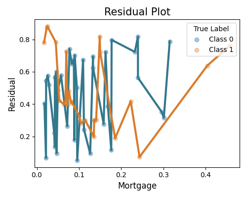
Residual analysis of the samples in that segment

exp.segmented_diagnose(model="XGB2", show="accuracy_residual",
                       segment_id=0, segment_method="auto", segment_feature="Balance",
                       show_feature="Mortgage", figsize=(5, 4))

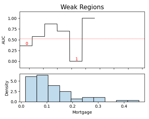
Weakspot analysis of the samples in that segment

exp.segmented_diagnose(model="XGB2", show="weakspot",
                       segment_id=0, segment_method="auto", segment_feature="Balance",
                       slice_features=["Mortgage"], metric="AUC", figsize=(5, 4))

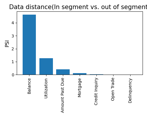
Distributional distance comparison between the specificed segment and the remaining (feature-by-feature)

res = exp.segmented_diagnose(model="XGB2", show="distribution_shift",
                             segment_id=0, segment_method="auto", segment_feature="Balance",
                             figsize=(5, 4), return_data=True)

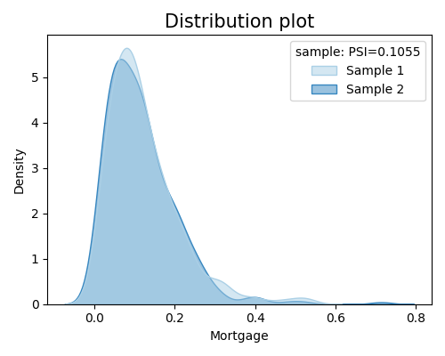
Distributional distance comparison between the specificed segment and the remaining (density of one selected feature)

res = exp.segmented_diagnose(model="XGB2", show="distribution_shift",
                             segment_id=0, segment_method="auto", segment_feature="Balance",
                             show_feature="Mortgage", figsize=(5, 4), return_data=True)

Estimated memory usage: 41 MB