2.7. Data Quality (Drift Test)

The last part of data quality is to compare the distribution between train and test sets, i.e., data drift test. Data drift refers to the phenomenon where the statistical properties of the data used for training a machine learning model change over time, leading to a mismatch between the training and test sets. In other words, the assumptions made during the model development, based on the training data, may no longer hold when the model is applied to new, unseen data.

Data drift can manifest in various ways, including changes in the distribution of feature values, shifts in the relationships between variables, or alterations in the frequency of certain patterns within the data. This discrepancy between the training and test sets can significantly impact the model’s performance and generalization ability. In PiML, we provide two data drift tests: marginal distribution drift and whole dataset energy distance.

2.7.1. Marginal Distribution Drift

This test evaluates the marginal distribution distance between the training and testing sets. For each feature, we provide three distance metrics:

• Population Stability Index (PSI): PSI is a statistical measure used to determine the extent to which the distribution of a variable has changed. It is a discrete (binned) version of the Kullback-Leibler (K-L) distance between two sets of sample data. More specifically, define a binning scheme that bins the two datasets \(P\) and \(Q\) into \(B\) bins. The discrete K-L distance between \(P\) and \(Q\) with respect to \(P\) is defined as \(D_{KL} (p│q)= \sum_{i=1}^B p_i ln ((p_i/q_i))\). Note that this distance is asymmetric. Define the distance with resect to \(q\) as \(D_{KL} (q│p)= \sum_{i=1}^B q_i ln (q_i/p_i)\). Then, PSI is the sum of the two asymmetric versions:

\[\begin{align} D(P, Q)_{PSI} = D_{KL}(p│q) + D_{KL} (q│p) = \sum^{B}_{i=1} (p_i - q_i)ln \frac{p_i}{q_i}. \end{align}\]

Here, \(B\) is the number of bins, and \(p_i\)’s and \(q_i\)’s are the proportions of the two samples in each bin. Note that the PSI calculation is related to the binning method, and PIML provides two options for binning, i.e., “equal width” or “equal quantile”. The number of bins is fixed at 10.

• Wasserstein distance 1D (WD1) distance: WD1 calculates the absolute difference between the cumulative distribution functions of the two samples.

\[\begin{align} D(F, G)_{WD1} = \int |F(x) - G(x)| dx. \end{align}\]

Here \(F(x)\) and \(G(x)\) are the cumulative distribution functions of the target and base population.

• Kolmogorov-Smirnov (KS) distance: KS calculates the maximum absolute distance between the cumulative distribution functions of the two samples. In PiML, the WD1 and KS statistics are calculated by the wasserstein_distance and ks_2samp functions from scipy.stats.

\[\begin{align} D(F, G)_{KS} = \sup_x |F(x) - G(x)|. \end{align}\]

The usage of this test is shown in the following example.

exp.data_quality(show="drift_test_distance", distance_metric="PSI",
                 psi_buckets="uniform", figsize=(5, 4))

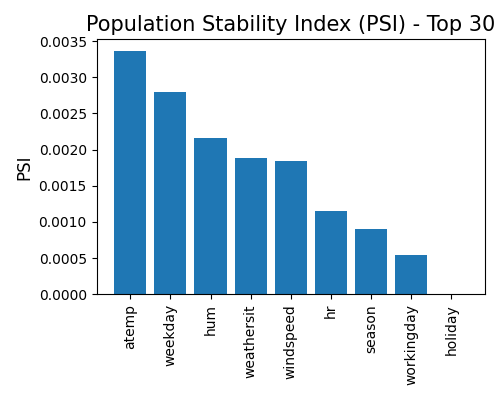
The additional argument distance_metric can be used to change the distance metric displayed on the plot, and psi_buckets is responsible for changing the binning method when calculating PSI. The default distance metric is PSI, and the default binning method is “uniform”. The distance metric can be set to “WD1” or “KS”, and the binning method can be set to “uniform” or “quantile”.

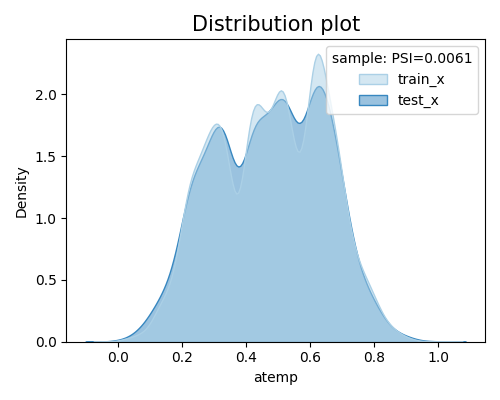
We can also compare the marginal densities of the train and test sets for a particular feature, by setting the show_feature argument to the name of the desired feature.

exp.data_quality(show="drift_test_distance", distance_metric="PSI", psi_buckets='quantile',
                 show_feature="atemp", figsize=(5, 4))

2.7.2. Energy Distance

Energy distance is a statistical measure used to quantify the dissimilarity or discrepancy between two probability distributions. It is commonly employed to assess the difference between the distributions of two sets of data points. This distance metric provides a way to evaluate how well one set of observations represents another, and it is particularly useful in comparing empirical distributions.

The energy distance of two samples \(x\) and \(y\) in high dimensional settings can be empirically estimated using the following formula:

\[\begin{aligned} D(x, y)_{\mathrm{E}} = \frac {2}{nm} \sum _{i=1}^{n} \sum _{j=1}^{m} \|x_{i}-y_{j}\| - \frac {1}{n^{2}} \sum _{i=1}^{n}\sum _{j=1}^{n}\|x_{i}-x_{j}\| - \frac {1}{m^{2}} \sum _{i=1}^{m}\sum _{j=1}^{m}\|y_{i}-y_{j}\|, \end{aligned}\]

where \(n\) is the size \(x\), and \(m\) is the size of \(y\). To speed up the computation, we randomly sample 10000 data points from the training and testing sets, respectively. The usage of this test is shown in the following example.

exp.data_quality(show="drift_test_info", figsize=(5, 4))

	Train Size	Test Size	Energy Distance
	13889	3476	0.000488

In the table, we displays the energy distance, as well as the size of training and testing samples. A zero energy distance indicates perfect similarity (i.e., the train and test distributions are identical) and higher values suggesting increasing dissimilarity.

2.7.3. Examples

The full example codes of this section can be found in the following link.

Example

• Data Quality Check