2.6. Data Quality (Outlier Detection)
In addition to the data integrity test, the subsequent component of data quality involves outlier detection. This submodule is designed to identify outliers following the data preparation step. The outcomes of this analysis provide users with valuable insights to pinpoint and eliminate outliers, thereby improving the quality and reliability of subsequent modeling tasks.
2.6.1. Methodology
Eight distinct outlier detection methods are provided, including Isolation Forest, Cluster-Based Local Outlier Factor (CBLOF), Principal Component Analysis (PCA), KmeansTree, K-Nearest Neighbor (KNN), Histogram-Based Outlier Detection (HBOS), One-Class SVM and Empirical Cumulative Distribution-based Outlier Detection (ECOD). All these methods are implemented in the piml.data.outlier_detection module. For each outlier detection estimator, the prediction output is the outlier score of each sample. The higher the outlier score, the more likely the sample is an outlier.
2.6.1.1. Isolation Forest
This algorithm adopts a unique approach to isolate observations by following a random selection process [Liu2008]. It begins by randomly choosing a feature from the dataset and then selecting a split value for that feature within the range of its maximum and minimum values. This process is repeated recursively to construct isolation trees, until the node has only one instance, or all data at the node have the same values.
The algorithm measures the anomaly score based on the average path length required to isolate each observation. Outliers are expected to have shorter average path lengths, indicating they are easier to separate from the rest of the data. In contrast, normal observations will require longer paths for isolation. The randomness in feature and split value selection contributes to the algorithm’s efficiency and ability to handle high-dimensional datasets. It does not rely on the specific distribution of the data, making it suitable for various types of data and outlier detection tasks. Note that the IsolationForest in PiML is a wrapper of sklearn’s implementation sklearn.ensemble.IsolationForest.
2.6.1.2. Cluster-Based Local Outlier Factor (CBLOF)
This method for outlier detection is based on cluster analysis, originally proposed by [He2003]. The process can be divided into the following steps:
Partition the data into clusters using K-means or Gaussian mixture model. Clusters can be classified into two categories, namely large clusters and small clusters, based on the size of each cluster. The size of a cluster is determined by the number of points it contains, and a given threshold is utilized for this classification.
Calculate the CBLOF score for each sample.
For samples belonging to large clusters, compute the Euclidean distance between each sample and its corresponding cluster centroid. This distance represents the outlier score for samples within large clusters.
For samples belonging to small clusters, calculate the Euclidean distance between each sample and the centroid of the nearest large cluster. This distance serves as the outlier score for samples within small clusters.
Multiplication by Cluster Size (optional): By default, the outlier score is not multiplied by the cluster size. However, if desired, the outlier score can be multiplied by the cluster size to emphasize the impact of outliers within larger clusters.
This method effectively utilizes the characteristics of clusters to detect outliers. The score calculation considers both the distances within a cluster and the relative distances to neighboring clusters. By combining these factors, the CBLOF score provides a comprehensive measure for identifying and quantifying outliers in the dataset. See more API details in CBLOF.
2.6.1.3. Principal Component Analysis
In addition to the clustering-based methods, dimensionality reduction techniques like Principal Component Analysis (PCA) can also be utilized for outlier detection. In PiML, there are two PCA-based methods for calculating the outlier score: Mahalanobis distance and error reconstruction, as elaborated in PCA.
Mahalanobis distance: This method computes the distance between each data point and the centroid of the dataset, taking into account the covariance structure of the data. The Mahalanobis distance accounts for correlations between variables and provides a measure of how far each data point deviates from the overall centroid. The Mahalanobis distance can be obtained easily with PCA under the formula, see [Shyu2003] for details.
where \(z_{i}\) are the \(i\)-th principal component scores, and \(\lambda_{i}\) is the \(i\)-th eigenvalue of the covariance matrix which can be explained as the variance. But this is precisely the sum of squared distances in the transformed PCA space, which gives us the desired result.
Error reconstruction: This method utilizes the reconstruction error obtained from reconstructing each data point using the principal components. The reconstruction error quantifies the dissimilarity between the original data point and its reconstructed representation. Higher reconstruction errors indicate potential outliers.
In PiML, the reconstruction is performed by fitting an XGBoost model between the principal components and the covariates. This model is then used to reconstruct the covariates \(X_{new}\). The difference between the original covariates and the reconstructed data is calculated as the reconstruction error, i.e., \(X - X_{new}\). Finally, we also calculate the Mahalanobis distance of the reconstruction error as the final outlier score, to account for the correlations among reconstruction errors. If the reconstruction errors of each feature are mutually independent, the outlier score reduces to the mean squared reconstruction error.
2.6.1.4. KmeansTree
This method is proposed by the PiML authors, it combines the advantages of the cluster-based method and PCA-based method. The algorithm follows the steps outlined below:
Iterative K-means Clustering: The dataset is split iteratively using the K-means clustering algorithm with K set to 2. This process continues until certain conditions are met, such as reaching the maximum depth, the maximum number of levels, or a specific distributional distance threshold between two child leaves.
PCA Error Reconstruction-based Outlier Detection: This step is the same as the algorithm described in the PCA-based method above, but it is performed for each cluster separately.
The KmeansTree method takes advantage of the splitting behavior of the K-means clustering algorithm and the dimensionality reduction capabilities of PCA. By combining these techniques and utilizing the Mahalanobis distance, it aims to effectively detect outliers in the data. The KmeansTree approach can enhance outlier detection performance by increasing the homogeneity of the data after clustering. For further details, please refer to the KMeansTree module in PiML.
2.6.1.5. K-Nearest Neighbor
While KNN is more commonly known for its use in classification and regression, it can also be adapted for outlier detection, see [Ramaswamy2000] and [Angiulli2002]. The idea is to consider data points that have fewer neighbors as potential outliers. Here’s a simple explanation of how KNN can be used for outlier detection:
Distance Calculation: As in the typical KNN algorithm, calculate the distances between a data point and all other points in the dataset using a distance metric such as Euclidean distance.
Sorting: Sort the distances in ascending order.
Thresholding: Consider the top ‘K’ distances, where ‘k’ is a user-defined parameter.
Aggregation: Calculate the largest / mean / median distance of the top ‘K’ distances. This value is used as the outlier score for the data point.
The rationale behind this approach is that outliers are expected to have fewer similar data points in their vicinity compared to the majority of the data. By setting an appropriate threshold and ‘k’ value, you can control the sensitivity of the outlier detection. For further details, please refer to the KNN module in PiML.
2.6.1.6. Histogram-based outlier detection
Histogram-based outlier detection is a method that relies on analyzing the distribution of data using histograms and identifying anomalies based on deviations from the expected patterns. Here’s a brief overview of how this approach works:
Histogram Binning: we create histogram binning for all features, and each data point is assigned to a specific bin based on its value.
Outlier Scoring: outlier scores are calculated using the frequencies of each bin, using the following formula:
where \(p\) is the number of features. \(f_j\) is the jth features’ density function. And \(\alpha\) serves as the regularizer to prevent overflow, by default, \(\alpha\) is set to 0.1. Data points that fall into bins with significantly lower frequencies than the majority of bins may be considered outliers.
The advantage of histogram-based outlier detection is that it provides a visual representation of the data distribution, making it easier to interpret and understand the characteristics of outliers. However, the effectiveness of this method depends on the appropriate selection of bin sizes and threshold values, which may require some tuning. This method might not capture complex relationships in high-dimensional data as effectively as some other advanced outlier detection techniques. For more information about the algorithm, refer to [goldstein2012]. For detailed information about the API, please see HBOS.
2.6.1.7. One Class SVM
One-class SVM (Support Vector Machine) is a machine learning algorithm commonly used for outlier detection, see the algorithm details in [Schölkopf2001]. Unlike traditional SVMs that are designed for binary classification tasks (e.g., separating data into two classes), One-Class SVM is trained only on the “normal” class, and its goal is to identify outliers or anomalies.
The key advantage of One-Class SVM is its ability to work well in high-dimensional spaces and to identify outliers even when the normal data distribution is not clearly defined. It is particularly useful in scenarios where normal data is prevalent, but outliers are rare and may exhibit different patterns.
However, it’s important to note that One-Class SVM requires careful parameter tuning, such as selecting the appropriate kernel and regularization parameters, to achieve optimal performance. The choice of kernel function (e.g., radial basis function, polynomial) can significantly impact the algorithm’s ability to capture the underlying structure of the data.
In PiML, we provide a wrapper of the OneClassSVM class in scikit-learn, see detailed information about the API in OCSVM.
2.6.1.8. Empirical Cumulative Distribution-based Outlier Detection
Empirical cumulative distribution Function is a non-parametric way to estimate the cumulative distribution function of a dataset. In the context of outlier detection, it can be used to identify data points that deviate from the expected cumulative distribution.
ECOD leverages the skewness of a distribution to assign outlier scores to each dimension. If a distribution is right-skewed, the outlier score is determined using the CDF. Conversely, if the distribution is left-skewed, the outlier score is derived from its complement 1-CDF. ECOD then aggregates the univariate outlier scores across all dimensions to obtain the overall outlier score. The outlier score for a sample \(x\) is calculated using the following formula:
where \(p\) is the number of features, and \(F_j\) is the empirical cumulative density function of the jth feature. Two skewness indicators are used: \(s_l\) and \(s_r\). If a distribution exhibits left skewness or no skewness, \(s_l\) is assigned a value of 1; otherwise, it is set to 0. Similarly, if a distribution displays right skewness or no skewness, \(s_r\) is set to 1; otherwise, it is assigned a value of 0.
For more information about the algorithm, refer to the publication [Li2021]. For detailed information about the API, see ECOD.
2.6.2. Analysis and Comparison
This subsection briefly introduces the usage of outlier detection methods in PiML. The function name is data_quality. The key parameters include:
method: The outlier detection method to be used, which needs to be an instance of IsolationForest, CBLOF, PCA, KMeansTree, KNN, HBOS, OCSVM and ECOD.show: The type of analysis to be performed.threshold: The threshold to decide whether a sample is an outlier.remove_outliers: If True, then the outliers will be removed from the dataset.
2.6.2.1. Outlier Score distribution
Here is an example of displaying the score distribution of the PCA-based outlier detection method. The keyword of this plot is “od_score_distribution”. The parameter threshold is used to decide whether a sample is an outlier, which is the quantile of the outlier score of all samples, within 0 and 1.
from piml.data.outlier_detection import PCA
exp.data_quality(method=PCA(), show='od_score_distribution', threshold=0.999)
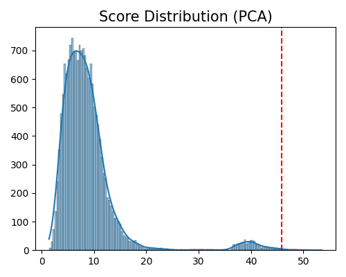
In this plot, the red dotted line represents the actual threshold of the outlier scores. Samples with outlier scores greater than this threshold are classified as outliers.
2.6.2.2. Marginal Distribution of Outliers
Here is an example of displaying the marginal distribution of detected outliers against a feature of interest. The keyword of this plot is “od_marginal_outlier_distribution”.
from piml.data.outlier_detection import PCA
exp.data_quality(method=PCA(), show='od_marginal_outlier_distribution', threshold=0.999)
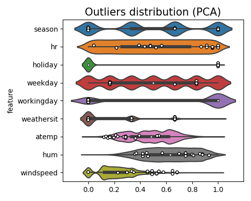
In this plot, a circle mark is used to indicate the presence of outliers. Although many of the outliers may fall within the normal range of individual features, they are still considered outliers in the context of the multivariate feature space. This phenomenon highlights the importance of considering the relationships and interactions between multiple features when identifying outliers.
2.6.2.3. Comparison of Different Methods
We use t-SNE to reduce the dimension of data to 2D for better visualization. Below is an example of comparing different methods, and the keyword of this plot is “od_tsne_comparison”.
from piml.data.outlier_detection import PCA, CBLOF
exp.data_quality(method=[PCA(), CBLOF()], show='od_tsne_comparison', threshold=[0.999, 0.999])
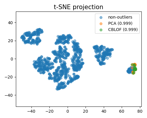
It is worth noting that, to mitigate the computational burden, the t-SNE algorithm used for visualization purposes is fitted using subsampled data. This subsampling technique allows for a representative subset of the data to be used, reducing the complexity of the t-SNE computation while still providing meaningful insights. In the plot mentioned above, the visualization reveals that the outliers detected by the two algorithms under comparison are noticeably distinct from each other. This discrepancy suggests that the algorithms may consider different aspects of the data when identifying outliers.
2.6.3. Examples
The full example codes of this section can be found in the following link.