2.8. Feature Selection
Feature selection aims at selecting a subset of covariates that are most relevant to the response. When the number of features is large, feature selection can help mitigate computational burden and avoid overfitting. Moreover, reducing the number of modeling features is also beneficial for enhancing model interpretability.
PIML has four built-in feature selection strategies. For demonstration purposes, we run the following example codes to initialize a PiML experiment for the BikeSharing dataset. Note that feature selection is based on training data, and hence the exp.data_prepare function should be executed before running exp.feature_select.
Warning
In all four strategies, we do not distinguish numerical features and categorical features. This treatment is not rigorous, especially for Pearson correlation, distance correlation, and rcit tests.
2.8.1. Correlations
Pearson correlation is a measure of the linear relationship between two continuous variables. Mathematically, the correlation coefficient of \(X\) and \(Y\) can be calculated in the following way.
The value of \(\rho_{X Y}\) ranges from -1 to 1, where the sign denotes the direction of the relationship, and the magnitude represents the correlation strength. The corresponding feature selection strategy is straightforward:
Calculate the Pearson correlation coefficient between each covariate and the response.
Select features with \(|\rho_{X Y}|\) greater than a user-specified
threshold.
These two steps are wrapped up and can be called in a single-line command in PiML, as follows,
exp.feature_select(method="cor", corr_algorithm="pearson", threshold=0.1, figsize=(5, 4))
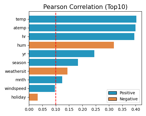
where “cor” is the keyword of the correlation strategy, “pearson” specifies the Pearson correlation, and 0.1 is the user-defined threshold. The output results include:
The upper-left figure shows the top 10 most important features, where the blue and orange bars denote the positive and negative correlations, respectively.
The upper-right table contains the correlation coefficients of all features.
The bottom line text highlights the selected features.
Pearson correlation is easy to compute and interpret. However, it cannot measure non-linear relationships, so its usage is limited. One can use the following three methods when dealing with more complex data relationships.
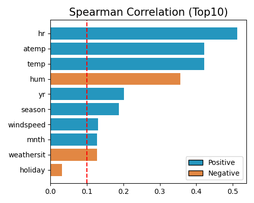
Spearman correlation is defined as the Pearson correlation between the ranks of the variables, which can be calculated as follows,
where \(\mathrm{R}(X), \mathrm{R}(Y)\) are the ranking variables of \(X, Y\), respectively. \(d_i=\mathrm{R}\left(X_i\right)-\mathrm{R}\left(Y_i\right)\) denotes the difference between the two ranks of the \(i\)-th observation. Spearman correlation measures the strength and direction of the relationship between two variables by evaluating how well the relationship between them can be described by a monotonic function. A perfect Spearman correlation of +1 or -1 occurs when each variable is a perfect monotonic function of the other, assuming there are no repeated data values. The corresponding feature selection strategy is similar to the Pearson correlation, except that we replace the keyword “pearson” with “spearman” in the corr_algorithm argument.
exp.feature_select(method="cor", corr_algorithm="spearman", threshold=0.1, figsize=(5, 4))
2.8.2. Distance Correlation
This is a measure of dependence between two paired random vectors. It can handle both linear and non-linear relationships. Given two features \(X\) and \(Y\), we first calculate their pairwise Euclidean distance matrix, as follows,
Then, these two matrices are centered,
The squared sample distance covariance is then defined as the arithmetic average of the products of \(A_{j, k}\) and \(A_{j, k}\)
Finally, the distance correlation between \(X\) and \(Y\) can be calculated via the following formula.
Similar to that of Pearson correlation, we first calculate the distance correlation of each covariate and the response and then use a threshold to determine which features are selected. Note that the distance correlation is always positive, ranging from 0 to 1, and hence we do not need to take the absolute value of these coefficients. In PiML, this method can be called using the following command,
exp.feature_select(method="dcor", threshold=0.1, figsize=(5, 4))
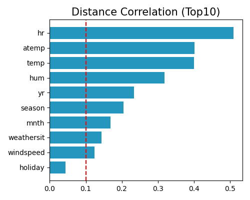
where the keyword is “dcor”.
The main advantage of distance correlation is that it can capture non-linear relationships. However, its calculation requires the pairwise distance matrix, which can be computationally very expensive when the sample size is large. To make the computation scalable for big data, we downsample 5000 samples from the original data and use them to calculate the distance correlation. The distance correlation is calculated using the statsmodels package by default. Alternatively, if the dcor package is installed, then the dcor package will be used automatically due to speed considerations.
2.8.3. Use of Feature Importance
This strategy is based on first fitting an ML model and using a post hoc method for selecting the important variables. It is composed of the following four steps:
Fit an XGB model using all the covariates and the response.
Run permutation feature importance test for the fitted XGB model, and get the importance of each feature.
Sort features in the descending order of importance (normalized such that all values sum to 1).
Select the top features with accumulated importance greater than a pre-defined threshold.
See the example usage below,
exp.feature_select(method="pfi", threshold=0.95, figsize=(5, 4))
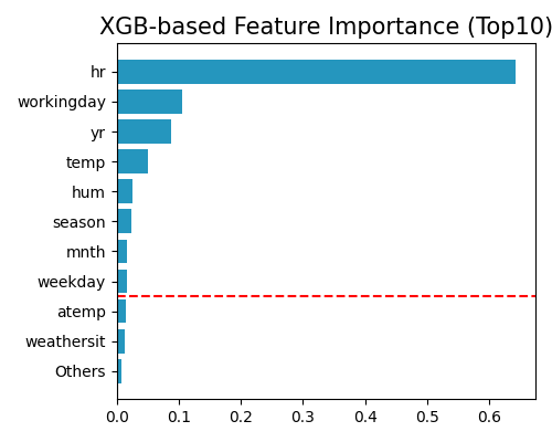
where the keyword here is “pfi”, and this test is based on the implementation of scikit-learn, and the details can be found at https://scikit-learn.org/stable/modules/generated/sklearn.inspection.permutation_importance.html. The setting threshold=0.95 means selecting the top features with the sum of feature importance greater than 95%. The valid range of threshold is 0 to 1, representing the percentage of accumulated importance. As we increase the threshold, more features would be selected.
By using XGB and PFI to rank features, the selected features are most relevant for predicting the response. There are several concerns with this approach: i) it is a post hoc method in that one has to fit a model first and use it to select the important variables; ii) the results can vary with the particular algorithm used; and iii) the fitted model can overfit or underfit, so the identified variables may not be the right ones.
2.8.4. Randomized Conditional Independence Test
This strategy aims to identify a Markov boundary of the response variable, where the Markov boundary is defined as the minimal feature subset with maximum predictive power. In particular, the randomized conditional independence test (RCIT) is used to test whether a variable is probabilistically independent of the response variable, conditioning on the Markov boundary. A forward-backward selection strategy is incorporated with RCIT to generate the Markov boundary.
2.8.4.1. RCIT Test
Given a Markov boundary set \(Z\), the goal is to test whether a feature \(X\) is independent of the response variable \(Y\), namely \(X \perp Y \mid Z\). The RCIT test is highly related to KCIT, see follows.
KCIT [Zhang2012]: kernel conditional independent test, works for non-linear and arbitrary data distribution; but not scalable.
RCIT [Strobl2019]: a fast approximation of KCIT; random Fourier features are used instead of reproducing kernel Hibert spaces.
Therefore, RCIT is used as it can handle non-linear relationships and is fast in computation (as compared to KCIT). A detailed introduction to RCIT is given below:
\(X, Y, Z\) are first transformed using random Fourier features;
Then the null hypothesis \(X \perp Y \mid Z\) is equivalent to zero partial cross-covariance \(\Sigma_{X Y \mid Z}=\Sigma_{X Y}-\Sigma_{Y Z} \Sigma_{Z Z}^{-1} \Sigma_{X Z}=0\);
The test statistics is then approximated by \(\left\|\hat{\Sigma}_{X Y \mid Z}\right\|_F^2=\mathrm{n} \hat{\Sigma}_{X Y}-\hat{\Sigma}_{Y Z}\left(\hat{\Sigma}_{Z Z}+\gamma I\right)^{-1} \hat{\Sigma}_{X Z}\);
The asymptotic distribution of the test statistics is \(\sum_{i=1} \lambda_i z_i^2\), where \(z_i\) are i.i.d. standard Gaussian variables.
Lindsay-Pilla-Basak (LPB; [Lindsayl2000]) approximates the CDF under the null using a finite mixture of Gamma distribution.
In PiML, the number of random Fourier features is set to 100 (\(Z\)) and 5 (\(X\) and \(Y\)), respectively.
2.8.4.2. Forward-Backward selection with Early Dropping (FBEDk):
The FBEDk [Borboudakis2019] algorithm is a combination of forward selection and backward elimination. Here we first run forward selection with a user-defined Markov boundary set as initial and then conduct backward elimination to further delete insignificant features.
Forward Selection
Given a predefined Markov boundary set, we initialize all the remaining covariate features as candidate features.
Run the RCIT test between each candidate feature and the response variable, conditional on the Markov boundary set.
Features with
p_value <= thresholdwill be selected as the candidate features.Among the candidate features, the most significant one will be added to the Markov boundary set.
Repeat the last three steps, and the algorithm stops as the candidate set is empty.
The above steps describe one run of the forward phase. To increase accuracy, the overall forward phase is repeated for k times, i.e., the character “k” in “FBEDk”. As recommended by [Yu2020], the forward phase is repeated twice, i.e., the value of k is 2, and you may change this parameter by specifying the argument n_forward_phase.
Backward Elimination
Temporarily remove feature \(j\) from the Markov boundary set.
Run RCIT test for feature \(j\) and \(Y\), conditional on the temporary Markov boundary set.
Permanently remove feature \(j\) from the Markov boundary set, if
p_value > threshold.
exp.feature_select(method="rcit", threshold=0.001, n_forward_phase=2, kernel_size=100, figsize=(5, 4))
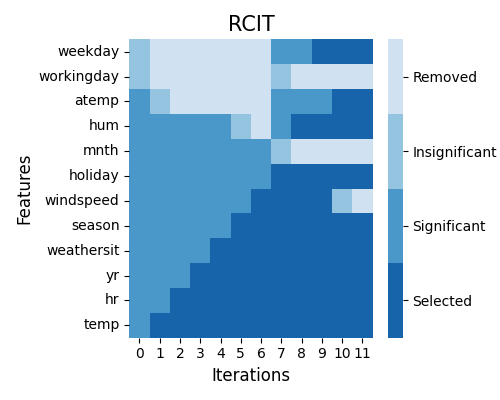
The keyword here is “rcit”. The upper-left figure shows the step-by-step formulation of the Markov boundary set. The value of the threshold should be between 0 to 1. The smaller its value, the fewer features would be marked as significant and then selected.
In the beginning, the Markov boundary set is empty, and the RCIT test is run over each feature and the response.
As shown in iteration zero, some features are marked as significant if the corresponding p_value <= threshold, e.g., hr and temp; while workingday and weekday are shown to be insignificant. In iteration one, the most significant feature temp is added to the Markov boundary set, while workingday and weekday are then removed from the candidate feature list. This procedure will be repeated, and in the end, seven features are selected, including, temp, hr, yr, weathersit, season, hum, and mnth.
As the FBEDk algorithm can start with an arbitrary Markov boundary set, users may define a non-empty Markov boundary set as the start point, see the following example.
exp.feature_select(method="rcit", threshold=0.001, preset=["hr", "temp"], figsize=(5, 4))
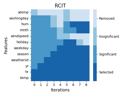
This time, two features hr and temp are selected as the initialization, and they are shown in deep blue in iteration 0.
The RCIT-based feature selection method is capable of handling non-linear relationships, and the selected features are all causally related to the response, subject to the pre-defined significance level. The disadvantages of this method include: a) the computational burden is relatively high; b) as it is a sequential selection approach, the results may be slightly different as we use different initial Markov boundary sets.
2.8.5. Examples
The full example codes of this section can be found in the following link.