4.3. Hstats (Friedman’s H-statistic)
H-statistic measures the interaction strength of two features [Friedman2008].
4.3.1. Algorithm Details
Consider a set of features, represented by \(X\), and a fitted model, represented by \(\hat{f}\). The H-statistic is defined based on partial dependence, as follows:
where feature \(j\) and \(k\) are two features in \(X\), \(x_j^{(i)}\) and \(x_k^{(i)}\) are the values of features \(j\) and \(k\) for the \(i\)-th sample, respectively, and \(PD_{jk}(x_j^{(i)}, x_k^{(i)})\) is the partial dependence of \(\hat{f}\) on features \(j\) and \(k\) at \((x_j^{(i)}, x_k^{(i)})\). The H-statistic is a measure of the interaction strength between features \(j\) and \(k\). The larger the H-statistic, the stronger the interaction between features \(j\) and \(k\). The H-statistic is symmetric, i.e., \(H_{jk}=H_{kj}\).
4.3.2. Usage
H-statistic can be calculated using PiML’s model_explain function. The keyword for PDP is “hstats”, i.e., we should set show = “hstats”. Additionally, the following arguments are relevant to this analysis:
use_test: If True, the test data will be used to generate the explanations. Otherwise, the training data will be used. The default value is False.sample_size: To speed up the computation, we subsample a subset of the data to calculate PDP. The default value is 2000. To use the full data, you can setsample_sizeto be larger than the number of samples in the data.grid_size: The number of grid points in PDP. The default value is 10.response_method: For binary classification tasks, the PDP is computed by default using the predicted probability instead of log odds; If the model does not have “predict_proba” or we setresponse_methodto “decision_function”, then the log odds would be used as the response.
The following code shows how to calculate the H-statistic of a fitted XGB2 model.
exp.model_explain(model="XGB2", show="hstats", sample_size=2000, grid_size=5,
                  figsize=(5, 4))

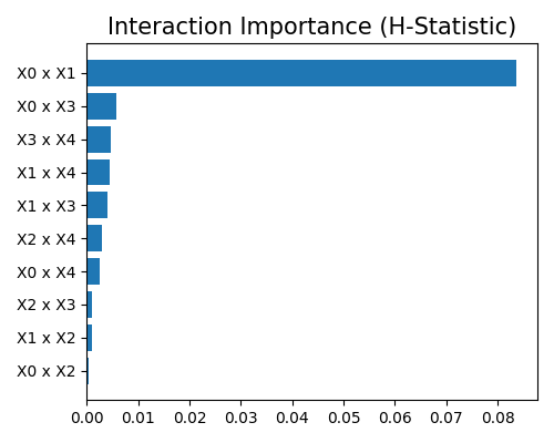
The plot above lists the top-10 important interactions. To get the H-statistic of the full list of interactions, we can set return_data=True, and the H-statistic of all interactions will be returned as a dataframe, as shown below.
result = exp.model_explain(model="XGB2", show="hstats", sample_size=2000, grid_size=5,
                           return_data=True, figsize=(5, 4))
result.data
