4.2. PDP (Partial Dependence Plot)¶

A partial dependence plot (PDP) [Friedman2001] is a model-agnostic tool that helps visualize the relationship between a subset of features and the predicted response. This allows us to determine whether the relationship between the target and an input feature is linear, monotonic, or more complex. However, one key assumption of PDP is that the features in the complement set are not correlated with the features of interest.

4.2.1. Algorithm Details¶

Consider a set of features, represented by \(X\), and a fitted model, represented by \(\hat{f}\). Note that for binary classification, we use the predicted log odds instead of the probability as the output function. Suppose we partition \(X\) into two sets: \(X_S\), which represents the features of interest, and \(X_C\), which represents the complement of \(X_S\). In this context, the partial function is defined as follows:

\[\begin{align} \mathrm{PD}_{S}(x_{S})=\mathbb{E}_{X_{C}}[\hat{f}(x_{S},X_{C})]= \int \hat{f}(x_{S}, X_{C})p(X_{C})dX_{C}, \tag{1} \end{align}\]

where the integral above can be approximated using the training data,

\[\begin{align} \mathrm{PD}_{S}(x_{S}) = \frac{1}{n}\sum_{i=1}^n \hat{f}(x_{S}, x_{C}^{(i)}), \tag{2} \end{align}\]

where \(x_{C}^{(i)}\) is the complement features of the \(i\)-th training sample. The integral approximation described above is commonly referred to as the “brute” method. However, for some tree-based estimators, a faster recursive method is also available. In PiML, the PDP is obtained by calling the partial_dependence function of the scikit-learn package; see more details here.

Warning

PDPs also have a few limitations, including:

Assumption of independence: PDPs assume that the features of interest are independent of each other. If the features are highly correlated, the results can be inaccurate, as they require extrapolation of the response at predictor values that are far outside the multivariate envelope of the training data.
Inconsistent global and local explanation: PDPs provide an average view of features’ effect on the predicted response. Local effects or effects specific to certain subsets of data may be different from global ones.

4.2.2. Usage¶

Visualizing PDPs using PiML is a straightforward process that can be accomplished with the model_explain function. The keyword for PDP is “pdp”, i.e., we should set show = “pdp”. Additionally, the following arguments are relevant to this analysis:

uni_feature: The name of the feature of interest for one-way PDPs.
bi_features: The names of the features of interest for two-way PDPs.
use_test: If True, the test data will be used to generate the explanations. Otherwise, the training data will be used. The default value is False.
sample_size: To speed up the computation, we subsample a subset of the data to calculate PDP. The default value is 2000. To use the full data, you can set sample_size to be larger than the number of samples in the data.
grid_size: The number of grid points in PDP. The default value is 100 for 1D PDP and 10 for 2D PDP.
response_method: For binary classification tasks, the PDP is computed by default using the predicted probability instead of log odds; If the model does not have “predict_proba” or we set response_method to “decision_function”, then the log odds would be used as the response.
sliced_line: A parameter for two-way PDP. If True, the two-way PDP will be visualized using sliced 1D line plot. Otherwise, the two-way PDP will be visualized using 2D heatmap. The default value is False.

For illustration purposes, we use PDPs to explain a fitted XGB2 model fitted on the BikeSharing dataset.

4.2.2.1. One-way PDPs¶

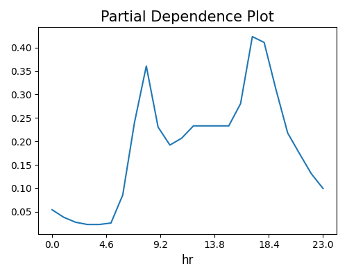
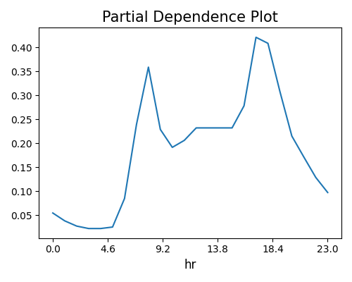
The one-way PDP describes the relationship between the predicted response and a single feature. To trigger one-way PDP, we need to specify a feature name in uni_feature. The following code shows how to visualize the one-way PDP for the numerical feature hr.

exp.model_explain(model="XGB2", show="pdp", uni_feature="hr", use_test=False,
                  grid_size=50, original_scale=True, figsize=(5, 4))

../../_images/sphx_glr_plot_1_pdp_001.png

The plot above suggests a non-linear relationship between the predicted response and the input feature of interest (hr). The grid_size parameter controls the number of grid points in PDP. The original_scale is set to True if we want to use the original scale of that feature.

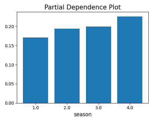
For categorical features, the PDP is a bar chart. The plot below indicates that bike sharing tends to be more substantial in the 4th season.

exp.model_explain(model="XGB2", show="pdp", uni_feature="season",
                  original_scale=True, figsize=(5, 4))

../../_images/sphx_glr_plot_1_pdp_002.png

4.2.2.2. Two-way PDPs¶

The two-way PDP shows the interaction between two features, which is useful for visualizing the joint effect of two features on the predicted response. To trigger two-way PDP, we need to specify two feature names in bi_features. The argument sample_size is used to speed up the computation of 2D PDP, which works by subsampling a subset of the data, and the default value is 2000. If the sample size is less than sample_size, then the entire training dataset will be used. In addition to the heatmap, we also provide an alternative sliced 1D plot, which can be triggered by setting sliced_line to True.

exp.model_explain(model="XGB2", show="pdp", bi_features=["hr", "workingday"],
                  grid_size=10, sample_size=10000, sliced_line=False, original_scale=True, figsize=(5, 4))

../../_images/sphx_glr_plot_1_pdp_003.png

The plot above shows the dependence of bike rental counts on the joint values of workingday and hr using a two-way PDP. We observe that the bike rental counts are higher during the working days (i.e., workingday = 1) than the non-working days (i.e., workingday = 0). The bike rental counts are also higher during the daytime than the nighttime. The interaction between workingday and hr is also observed in the plot.