4.6. LIME (Local Interpretable Model-Agnostic Explanation)
LIME (Local Interpretable Model-Agnostic Explanation; [Ribeiro2016]) is a model agnostic explanation tool. It does so by creating a surrogate interpretable model, such as a Lasso or decision tree, to explain how the original model makes predictions for a given input sample.
4.6.1. Algorithm Details
The process is straightforward:
Create a simulated dataset by randomly perturbing the input sample with noises (as \(x\)), and then evaluate the output of the original model on these perturbed samples (as \(y\)).
An interpretable model (Lasso in our case) is fitted on this simulated data, with weights assigned to each perturbed sample based on its proximity to the original input sample.
The PiML implementation of LIME is based on the LIME package. For binary classification problems, it uses predict_proba as the response.
Warning
The explanation of two very close points varied greatly in a simulated setting. In addition, the randomness during the sampling may lead to different LIME interpretations if we repeat the sampling process. Therefore, we must use our judgment to see if the result makes sense.
4.6.2. Usage
The LIME explanation is also integrated into the model_explain function of PiML, with the keyword “lime” for the argument show.
use_test: If True, the test data will be used to generate the explanations. Otherwise, the training data will be used. The default value is False.sample_id: The sample index in the train / test set, and the default value is 0. If use_test = True, the valid values is from 0 to test_sample_size - 1; otherwise, it ranges from 0 to train_sample_size - 1.centered: If True, the data will be centered, which means we contrast its effect against with the population mean. The default value is True.
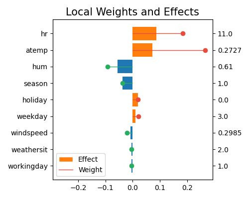
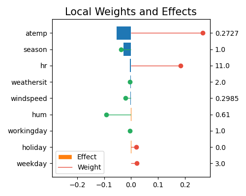
Below, we will demonstrate how to use LIME to explain the first training sample (sample_id=0) of a fitted XGB2 model on the BikeSharing dataset. In particular, we compare the centered and uncentered results by setting centered to True and False, respectively.
Uncentered predictors
exp.model_explain(model="XGB2", show="lime", sample_id=0, centered=False,
                  original_scale=True, figsize=(5, 4))

This plot is similar to the local interpretation of GLM, as we use Lasso as the surrogate model. The stems represent the coefficients and the bars show the effect. It shows the linear regression coefficients and marginal effects of the top-10 features (with feature values on the right axis) that contribute to the prediction of bike counts. The Weight represents the regression coefficients, and Effect represents the marginal effects. From top to bottom, hr contributes the most to the prediction of bike counts, followed by atemp, then hum, and so on. Note that this plot only shows the top 10 features with the largest contributions. To get the full results, you can set the parameter return_data to True.
Centered predictors
Centering is crucial when group effects are of interest and can be done by subtracting the mean attribute from each attribute element.
exp.model_explain(model="XGB2", show="lime", sample_id=0, centered=True,
                  original_scale=True, figsize=(6,5))

By centering the data and calculating the marginal effects, the model itself remains unchanged, but the interpretation of the marginal effects may change significantly, as we are essentially comparing the contribution of each feature to the average population, rather than the individual sample values. For instance, hr has a large contribution to the prediction in the uncentered data. However, when the data is centered, its contribution becomes negligible. This is because the feature value of this sample (11 am) is close to the population mean, and its contribution is now mainly captured by the intercept term.
