4.4. ICE (Individual Conditional Expectation)
Individual Conditional Expectation (ICE) plots [Alex2015] and PDPs both visualize the relationship between a feature of interest and the predicted response. However, ICE plots focus on the dependence of the predicted response on the feature for each instance, while PDPs show the average effect of the feature on the response across all instances in the dataset.
4.4.1. Algorithm Details
Let \(X\) represent the set of input features of a predictor function, and \(\hat{f}\) be a fitted model to be explained. We partition \(X\) into two sets, i.e., \(X_{S}\) (features of interest) and its complement \(X_{C}\). To be specific, an ICE plot for a feature \(x_{S}\) and an instance \(i\) can be defined as:
Let \(X\) denote the set of input features for a predictor function, and \(\hat{f}\) be a fitted model that needs to be explained. We partition \(X\) into two subsets, namely \(X_{S}\) (the features of interest) and its complement \(X_{C}\). Specifically, an ICE plot for a feature \(x_{S}\) and an instance \(i\) is defined as follows:
In PiML, the ICE plot is implemented using the scikit-learn package. For a more detailed analysis of this algorithm, please refer to the documentation available here.
Note
For binary classification tasks, the ICE is computed by default using the predicted probability instead of log odds. In exp.model_explain, there exist an argument called response_method. If we want to use the predicted probability as the output, we can set response_method to “decision_function”.
4.4.2. Usage
Below we still use a fitted XGB2 model on the BikeSharing dataset for illustration. The show parameter needs to be “global_ice”, and the following parameters are also related to ICE plots:
uni_feature: The name of the feature of interest for one-way ICE.use_test: If True, the test data will be used to generate the explanations. Otherwise, the training data will be used. The default value is False.sample_size: To speed up the computation, we subsample a subset of the data to calculate ICE. The default value is 2000. To use the full data, you can setsample_sizeto be larger than the number of samples in the data.grid_size: The number of grid points in ICE. The default value is 100 for 1D ICE.response_method: For binary classification tasks, the ICE is computed by default using the predicted probability instead of log odds; If the model does not have “predict_proba” or we setresponse_methodto “decision_function”, then the log odds would be used as the response.
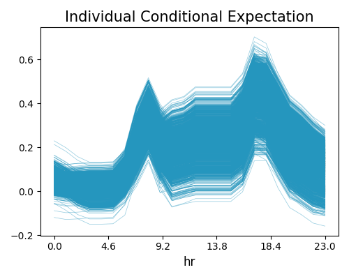
The code snippet below provides an example of how to generate an ICE plot using PiML. The uni_feature parameter is set to “hr”. This configuration will produce a line plot, with each line representing an instance in the dataset. The plot shows how the predicted response varies when the value of “hr” changes, while all other features remain constant. By examining the individual lines in the ICE plot, we can better understand how the model makes predictions for each instance in the dataset. We can also identify any patterns or interactions that may be relevant to our analysis.
exp.model_explain(model="XGB2", show="ice", uni_feature="hr", original_scale=True, figsize=(6, 5))

From the plot, we observe a similar pattern as the value of hr increases for all instances, which is also consistent with the PDP plot generated in the previous section. The predicted values are generally lower when hr is less than 4.6. For values of hr between 4.6 and 8.3, and between 10 and 18, most of the instances record an increase in prediction as the value of hr increases. Apart from that, we also observe that the bandwidth of the predicted response is much larger as hr is greater than around 9. This indicates that the rest variables have more contributions to the final prediction during that period of the day.
