4.5. ALE (Accumulated Local Effects)
Accumulated Local Effects (ALE; [Apley2016]) is a model-agnostic method for explaining how features impact a model’s prediction. Its aim is similar to that of PDP, but PDP results may be biased when features are correlated. ALE overcomes this limitation and offers a quicker and unbiased alternative to PDP.
4.5.1. Algorithm Details
ALE plots, by definition, accumulate the local effects over the range of features. Here we just describe the one-way ALE for a single numerical feature, i.e., one-way ALE. It first divides the feature of interest into \(K\) intervals (bins). The local effect of each bin is computed as the difference in prediction between the first and last values. Let \(N_{j}(k) = (z_{k-1,j} , z_{k,j}]\) be the \(k\)-th interval for the \(j\)-th feature. The split point \(z_{k,j}\) is usually set as the \(\frac{k}{K}\) quantile of the \(j\)-th feature. Based on the binning results, we can compute the uncentered effect of the feature \(j\) as follows:
\[\begin{align} \hat{h}_{j,ALE}(x) = \sum_{k=1}^{k_{j}(x)}\frac{1}{n_{j}(k)}\sum_{i:x_{j}^{(i)}\in N_{j}(k)}[\hat{f}(z_{k,j},\textbf{x}_{-j}^{(i)})- \hat{f}(z_{k-1,j},\textbf{x}_{-j}^{(i)}))], \tag{1} \end{align}\]
where \(k_{j}(x)\) is the index of the interval, \(n_{j}(k)\) is the number of samples in \(N_{j}(k)\), and \(\hat{f}\) is the model being explained. Finally, the ALE is centered using the following formula:
Note that the computation of ALE is faster than that of PDP, as it requires less number of function calls to \(\hat{f}\). Moreover, there is no standard for selecting the number of intervals. If the number of intervals is too small, the ALE plots might not be very accurate. On the other hand, If the number is too high, the curve will have many small ups and downs. For additional details on the two-way ALE, please refer to the original paper [Apley2016]. In PiML, the ALE plot is generated based on the Python package PyALE.
Warning
When features are strongly correlated, it is not suggested to do the interpretation of the effect across intervals. That is because the effects are computed per interval (locally), and require no extrapolation beyond the data envelope. If fix one feature and move another feature (highly correlated with the fixed one) from one interval to another one, the model being explained \(\hat{f}\) may output unreliable predictions, which will lead to unreliable ALE values. In other words, the ALE values are not reliable when the model is extrapolating outside of the data envelope. Therefore, as features are strongly correlated, we should interpret ALE plots locally for each bin.
4.5.2. Usage
This section illustrates how to use PiML to get the ALE plots. Similar to the visualization of PDPs, the visualization of ALE plots in PiML can be done using the model_explain function. The keyword for ALE plot is “ale”, i.e., we should set show = “ale”. Additionally, the following arguments are relevant to this analysis:
uni_feature: The name of the feature of interest for one-way ALE.bi_features: The names of the features of interest for two-way ALE.use_test: If True, the test data will be used to generate the explanations. Otherwise, the training data will be used. The default value is False.sample_size: To speed up the computation, we subsample a subset of the data to calculate ALE. The default value is 2000. To use the full data, you can setsample_sizeto be larger than the number of samples in the data.grid_size: The number of grid points in ALE. The default value is 100 for 1D PDP and 10 for 2D ALE.response_method: For binary classification tasks, the ALE is computed by default using the predicted probability instead of log odds; If the model does not have “predict_proba” or we setresponse_methodto “decision_function”, then the log odds would be used as the response.sliced_line: A parameter for two-way ALE. If True, the two-way ALE will be visualized using sliced 1D line plot. Otherwise, the two-way ALE will be visualized using 2D heatmap. The default value is False.
For illustration purposes, we fitted the ReLUDNN model on the Bike Sharing dataset.
4.5.2.1. One-way ALE
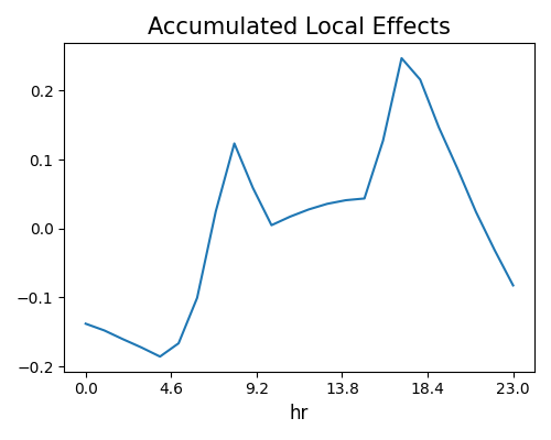
The one-way ALE tells us about the relationship between the target response and an input feature of interest. To generate an ALE plot of a single feature, we should specify the feature’s name in uni_feature. The grid_size parameter can be used to adjust the number of grid points in the plot.
exp.model_explain(model="ReLUDNN", show="ale", uni_feature="hr",
                  grid_size=50, original_scale=True, figsize=(5, 4))

The hourly bike counts have two peaks in the rush hours of the day, which is consistent with that of PDP. From the plot, we can see that the range of ALE values is centered around zero, this is because the ALE plot is centered using the mean of the local effects.
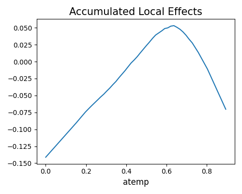
In addition to the feature hr, we also draw the ALE plot for the feature atemp, as shown below.
exp.model_explain(model="ReLUDNN", show="ale", uni_feature="atemp",
                  grid_size=50, original_scale=True, figsize=(5, 4))

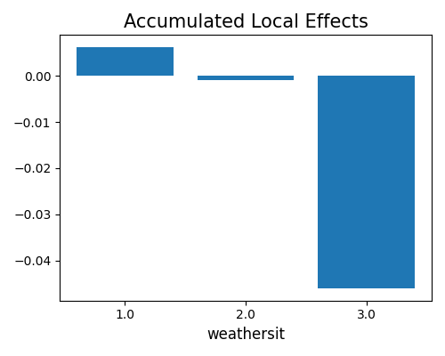
The plot above shows that the bike sharing counts reach the highest as atemp is around 0.6. The ALE plot is also centered around zero, which is consistent with the previous plot. ALE plot also supports categorical features. As the categorical feature has no ordering, we need to create an ordering for each category. In specific, we order the categories by their similarity (or distance) based on the rest features. Once we have the distances between all categories, we can reduce the pairwise distance matrix to a distance-vector, in which each element represents the distance score of a category. After that, we can order the categories using the distance score, and then calculate the ALE just like the numerical features.
exp.model_explain(model="ReLUDNN", show="ale", uni_feature="weathersit",
                  original_scale=True, figsize=(5, 4))

This is the ALE plot for the categorical feature weathersit. From this plot, we can see that weathersit with values 3 (Light Rain, etc) and 4 (Heavy Rain, etc) have a significantly negative effect on the final prediction, as compared to 1.0 (Clear, etc). Although the simple average of these four bars is negative, the average ALE over the full sample is still zero. That is because the density of category 1.0 is much larger than that of 3.0 and 4.0.
4.5.2.2. Two-way ALE
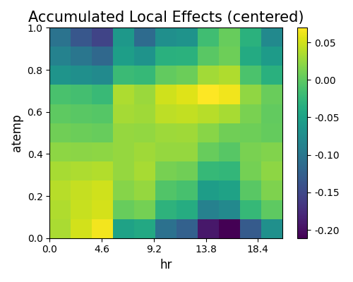
The two-way ALE (two inputs features of interest) shows the interaction between the two features. It estimates the interaction effect of two features, excluding the individual main effects. Technically, this is done by first estimating the uncentered two-way ALE, and then estimating and subtracting the main effects for the uncentered two-way ALE (instead of the model being explained). To generate ALE for two features, we will need to specify the bi_features parameter with two feature names. Similar to two-way PDP, you may view the two-way ALE using sliced 1D line plot by setting sliced_line=True.
exp.model_explain(model="ReLUDNN", show="ale", bi_features=["hr", "atemp"]
                  grid_size=10, sliced_line=False, original_scale=True, figsize=(5, 4))

In the plot above, lighter shade indicates an above average, while darker shade indicates a below average. In addition to adjusting for the overall mean effect, two-way ALE also adjusts for the main effects of both features. Therefore, the two-way ALE plot can be quite different from the two-way PDP, and one must keep the main effects in mind during the interpretation.
