5.7. Explainable Boosting Machines
An explainable boosting machine (EBM) proposed by [Lou2013] is another algorithm to fit generalized additive model and functional pairwise interactions:
where each main effect \(h_{j}(x_{j})\) or pairwise interaction \(f_{jk}(x_{j}, x_{k})\) is estimated via gradient boosted shallow trees, which is modified from the standard gradient boosting model. The training algorithm of EBM is divided into the following two steps: 1) Fit main effects by shallow-tree boosting in round-bin fashion; 2) Fit pairwise interactions on residuals, by
Detect interactions by a FAST algorithm (details in [Lou2013]).
For each interaction \((x_{j}, x_{k})\), model it by a depth-2 tree, either 1 cut in \(x_{j}\) and 2 cuts in \(x_{k}\), or 2 cuts in \(x_j\) and 1 cut in \(x_{k}\) (pick the better one).
Iteratively fit all the detected interactions until convergence.
The estimated shape functions by EBM are all piecewise constant. EBM is interpretable by visualizing the main effects and pairwise interactions, which is a key advantage over black-box models.
5.7.1. Model Training
PiML integrates the ExplainableBoostingRegressor and ExplainableBoostingClassifier by the interpret package, developed by Microsoft Research [Nori2013]. Here, we use the California Housing dataset as an example to demonstrate how to use it in PiML, as follows.
from piml.models import ExplainableBoostingRegressor
exp.model_train(model=ExplainableBoostingRegressor(interactions=10), name="EBM")
In EBM max_iter, max_bins, and learning_rate are the most important hyperparameters.
interactions: the maximum number of pairwise interactions to include, by default 10. Increasing this value will increase the model complexity and hence prediction performance. However, it may also lead to overfitting and a sacrifice of model interpretability.learning_rate: the learning rate of boosting, by default 0.01. Increasing the learning rate can lead to faster convergence, but may also lead to underfitting.max_bins: the max number of binning per feature, by default 256. By using a relatively small number of bins, EBM can be more robust to outliers and missing values.
5.7.2. Global Interpretation
Similar to the rest of GAMI models like XGB2 and GAMI-Net, EBM can be interpreted from various perspectives.
5.7.2.1. Main Effect Plot
The main effect plot in EBM, like GAM, displays the estimated effect of \(\hat{h}_{j}(x_{j})\) against \(x_{j}\). The main effect can be of any shape, and hence it is also called shape function. In EBM, the shape function is piecewise constant, as it is estimated by the shallow trees. To generate main effect plots in EBM, use the keyword “global_effect_plot” and specify the feature name with uni_feature.
exp.model_interpret(model="EBM", show="global_effect_plot", uni_feature="hr",
                    original_scale=True, figsize=(5, 4))
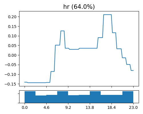
The figure above shows the estimated shape functions for the feature hr, together with the histogram plot on the bottom. The shape function is piecewise constant, and the number of bins is upper bounded by the hyperparameter max_bins. It can be observed that there exist 2 peaks of bike sharing around 8 AM and 5 PM, which correspond to the rush hour in a day.
5.7.2.2. Interaction Plot
To visualize the estimated pairwise interaction, we can still use the keyword “global_effect_plot” together with the feature names specified in bi_features.
exp.model_interpret(model="EBM", show="global_effect_plot", bi_features=["hr", "season"],
                    original_scale=True, figsize=(5, 4))
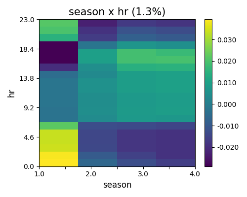
The figure above shows the estimated pairwise interaction between hr and season. The interaction captures the main effects’ residual pattern, and somehow, can be interpreted as the correction to the prediction of the main effects. For instance, it can be observed that there exists a minor positive effect at the night hours (around 7 pm to 7 am) of spring.
5.7.2.3. Effect Importance
The effect importance is calculated as the variance of the estimated shape functions, which is similar to the feature importance in GAM. The effect importance can be calculated for both main effects and pairwise interactions, using the keyword “global_ei”.
exp.model_interpret(model="EBM", show="global_ei", figsize=(5, 4))
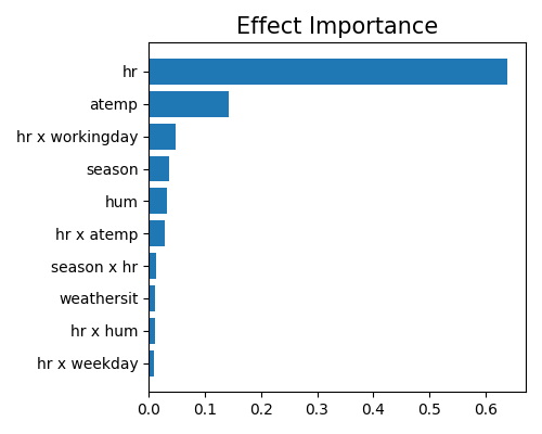
It can be observed that the main effect of hr is the most important, followed by atemp and the pairwise interaction between hr and workingday. Here we only plot the top-10 effect importance. Note that this plot only shows the top 10 effects with the largest importance. To get the full results, you can set the parameter return_data to True.
5.7.2.4. Feature Importance
As a GAMI model, the calculation of feature importance in EBM is the same as that of the XGB2 model, and we also use the keyword “global_fi” to draw the feature importance plot.
exp.model_interpret(model="EBM", show="global_fi", figsize=(5, 4))
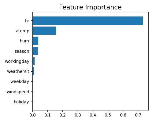
From this plot, we can observe that the two features hr and atemp take the dominant role in the model, followed by season and hum. The findings are quite close to that of the XGB2 model, as they share a similar model structure. Note that this plot only shows the top 10 features with the largest importance. To get the full results, you can set the parameter return_data to True.
5.7.3. Local Interpretation
The local interpretation of EBM also includes two parts: local feature contribution and local effect contribution. As a GAMI model, it also reveals how the final prediction is obtained by the main effects and pairwise interactions.
5.7.3.1. Local Effect Contribution
We use “local_ei” to draw the effect contribution of a given sample.
exp.model_interpret(model="EBM", show="local_ei", sample_id=0, original_scale=True, figsize=(5, 4))
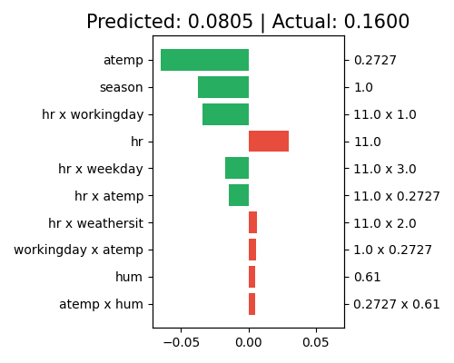
The right axis of the plot displays the predictor values for each effect, while the left axis shows the corresponding effect names. The title indicates that the predicted value for this sample is 0.0818, which differs slightly from the actual response of 0.16. The main effect of atemp makes the largest contribution to the final prediction, with a negative effect (approximately -0.06). The main effect of season and the pairwise interaction (hr and workingday) also have negative effects on the final prediction, following atemp. Note that only the top 10 effects with the largest contribution are shown in this plot. To see the complete results, set the return_data parameter to True.
5.7.3.2. Local Feature Contribution
The definition of feature contribution is the same as that of the XGB2 model. Similarly, we use the keyword “local_fi” to generate this plot, as follows.
exp.model_interpret(model="EBM", show="local_fi", sample_id=0, original_scale=True, figsize=(5, 4))
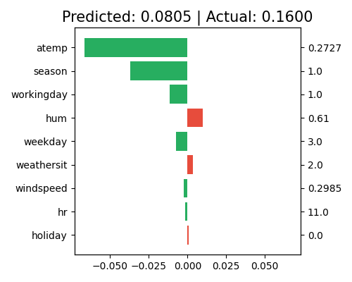
The feature contribution plot has a similar interpretation to that of the local effect contribution plot, but it displays the contribution by feature instead of by effect. For this sample, the main effects of atemp and season still have negative contributions to the final prediction. However, the contribution of feature hr almost equals zero at the feature level, in contrast to the significant positive contribution of its main effect. Note that only the top 10 features with the largest contribution are shown in this plot. To view the complete results, set the return_data parameter to True.
