5.8. GAMI-Net
The generalized additive model with structured pairwise interactions network (GAMI-Net; [Yang2021b]) is a neural network reformulation of the GAMI model, like XGB-2 and EBM.
GAMI-Net is a disentangled feedforward network with multiple additive subnetworks; each subnetwork consists of multiple hidden layers and is designed for capturing one main effect or one pairwise interaction. Several interpretability aspects are further considered,
Sparsity, to select the most significant effects for parsimonious representations;
Heredity, a pairwise interaction could only be included when at least one of its parent main effects exists;
Marginal clarity, to make main effects and pairwise interactions mutually distinguishable. (similar to the purification of XGB2)
Monotonicity: certain features can be constrained to be monotonic increasing or decreasing, which is achieved by imposing regularization during network training.
The training of GAMINet can be divided into the following three steps:
Train the main effect subnetworks and prune the trivial ones by validation performance.
Train pairwise interactions on residuals, by 1) Select candidate interactions by heredity constraint; 2) Evaluate their scores (by FAST) and select top-K interactions; 3) Train the selected two-way interaction subnetworks; 4) Prune trivial interactions by validation performance.
Retrain main effects and interactions simultaneously for fine-tuning network parameters.
Compared to XGB2 and EBMs, GAMI-Net has a continuous and smooth shape function, which is more interpretable. Also, it is very flexible to incorporate various interpretability constraints in neural networks.
5.8.1. Model Training
Here, we use the Bike Sharing dataset as an example to demonstrate how to use GAMI-Net in PiML. Similar to the rest interpretable models, GAMI-Net can be fitted and registered using the model train API.
from piml.models import GAMINetRegressor
exp.model_train(model=GAMINetRegressor(), name="GAMI-Net")
For the full list of hyperparameters, please see the API of GAMINetRegressor and GAMINetClassifier.
5.8.2. Global Interpretation
The inherent interpretation of GAMI-Net includes the main effect plot, pairwise interaction plot, effect importance plot, and feature importance plot.
5.8.2.1. Main Effect Plot
The main effect plot in GAMI-Net shows the estimated effect \(\hat{h}_{j}(x_{j})\) against \(x_{j}\). The main effect is piecewise linear, as we use ReLU activation functions. In PiML, we can use the keyword “global_effect_plot” to draw main effect plots, together with the argument uni_feature which takes the feature name as input.
exp.model_interpret(model="GAMI-Net", show="global_effect_plot", uni_feature="hr",
                   original_scale=True, figsize=(5, 4))
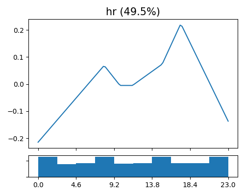
The figure above shows the estimated shape functions for the feature hr, together with the histogram plot on the bottom. Consistent with other interpretable models, it is found that there exist 2 peaks of bike sharing around 8 AM and 5 PM, which correspond to the rush hour in a day. The key difference between GAMI-Net and other interpretable models (XGB2 and EBM) is that the estimated shape function is continuous and smooth, which is a favorable feature for model interpretation.
5.8.2.2. Interaction Plot
To visualize the estimated pairwise interaction \(\hat{f}_{jk}(x_{j},x_{k})\) against \(x_{j}\) and \(x_{k}\), we can still use the keyword “global_effect_plot” together with the feature names specified in bi_features.
exp.model_interpret(model="GAMI-Net", show="global_effect_plot", bi_features=["hr", "weekday"],
                    original_scale=True, figsize=(5, 4))
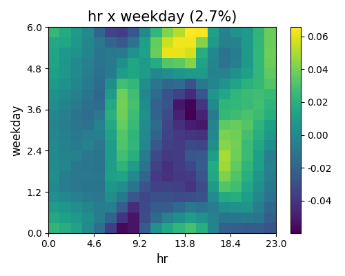
The figure above shows the estimated pairwise interaction between hr and weekday. From the plot, we find that there is a positive effect (+0.07) for bike sharing at 2 pm on Saturday and Sunday, and also some negative effect (-0.06) at 2 pm from Monday to Friday.
5.8.2.3. Effect Importance
The effect importance is calculated as the variance of the estimated shape functions, both for main effects and pairwise interactions.
exp.model_interpret(model="GAMI-Net", show="global_ei", figsize=(5, 4))
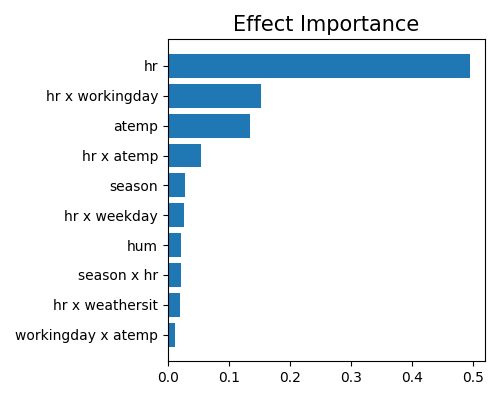
Here we only plot the top-10 effect importance. It can be observed that the main effect of hr is the most important, followed by the pairwise interaction between hr and workingday. This result is slightly different from that of XGB2 and EBM. Note that this plot only shows the top 10 effects with the largest importance. To get the full results, you can set the parameter return_data to True.
5.8.2.4. Feature Importance
As a GAMI model, the calculation of feature importance in GAMI-Net is the same as that of the XGB2 model. We use the keyword “global_fi” to draw the feature importance plot.
exp.model_interpret(model="GAMI-Net", show="global_fi", figsize=(5, 4))
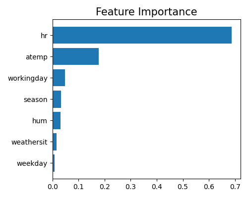
From this plot, we can observe that the top-3 important features are hr, atemp, and workingday. Note that this plot only shows the top 10 features with the largest importance. To get the full results, you can set the parameter return_data to True.
5.8.3. Local Interpretation
Similar to other GAMI models, the local interpretation of GAMI-Net consists of two components: local feature contribution and local effect contribution, which provide insight into how the final prediction is generated through the main effects and pairwise interactions.
5.8.3.1. Local Effect Contribution
We use “local_ei” to draw the effect contribution of a given sample.
exp.model_interpret(model="GAMI-Net", show="local_ei", sample_id=0, original_scale=True, figsize=(5, 4))
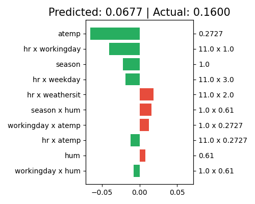
The right axis of the plot displays the predictor values for each effect, while the left axis shows the corresponding effect names. The title indicates that the predicted value for this sample is 0.0324, which differs from the actual response of 0.16. The main effect of atemp makes the largest contribution to the final prediction, with a negative effect (approximately -0.06). The pairwise interactions (hr, workingday), (hr, windspeed), and (hr, weekday) also have negative effects on the final prediction, following atemp. Note that only the top 10 effects with the largest contribution are shown in this plot. To see the complete results, set the return_data parameter to True.
5.8.3.2. Local Feature Contribution
The local feature contribution is also based on the aggregated contribution of each feature, which sums the effect of a feature over its main effect and all related pairwise interactions. Also, see the definition in the XGB2 model.
exp.model_interpret(model="GAMI-Net", show="local_fi", sample_id=0, original_scale=True, figsize=(5, 4))
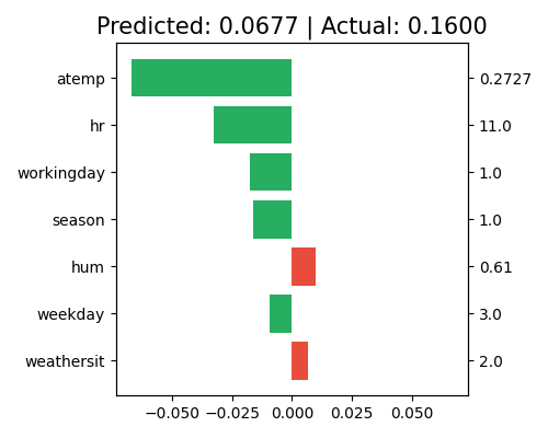
This plot displays the contribution at the feature level. For this chosen sample (sample_id = 0), the top-5 features (atemp, hr, workingday, season, windspeed) all have negative contributions to the final prediction. Although the main effect of hr is small, the aggregated effects of its related pairwise interactions make it the second important feature for this specific sample. Note that only the top 10 features with the largest contribution are shown in this plot. To view the complete results, set the return_data parameter to True.
