5.4. Fast Interpretable Greedy-tree Sums

Fast Interpretable Greedy-tree Sums (FIGS; [Tan2022]) is a recently proposed machine-learning algorithm that extends classification and regression trees (CART). FIGS can also be viewed as a special case boosted tree model, as a fitted FIGS usually consists of multiple additive trees. The prediction of a fitted FIGS is a linear combination of the predictions of all trees, as follows,

\[\begin{align} g(\mathbb{E}(y|\textbf{x})) = \mu + \sum_{k=1}^K f_k\left(\mathbf{x}\right), \tag{1} \end{align}\]

where \(\mu\) is the intercept, \(K\) is the number of trees, and \(f_k\) is the function of the \(k\)-th tree. The process of model fitting begins by estimating the intercept term through the average of the response variable. Next, the additive trees are fitted in a greedy manner using the (pseudo) residuals. It is important to note that the value of \(K\) is not a hyperparameter specified by the user but is instead determined during the model fitting process. The advantages of FIGS are summarized below.

• Compared with CART, FIGS has a more expressive model form, and also its predictive performance. CART is a single tree, while FIGS is an ensemble of multiple trees.

• Compared with boosted trees, FIGS can have a larger search space, given the same number of split iterations. In boosted trees, the search space is limited to boosting a new tree. In contrast, FIGS can either boost a new tree or grow existing trees, whichever reduces the loss most. However, the training of FIGS is slower than that of boosted trees, especially when the number of split iterations is large.

• The fitted model can be easily interpretable if the value of \(K\) is small. In practice, we usually limit the maximum iteration of FIGS to be within 1000.

5.4.1. Model Training

The authors of FIGS provided a Python implementation in the imodels package. In PiML, we re-implement this model, which is much faster and with more interpretation functionalities, see the corresponding API reference in FIGSRegressor and FIGSClassifier.

The training of FIGS is similar to that of the other interpretable models, as shown below.

from piml.models import FIGSRegressor
exp.model_train(model=FIGSRegressor(max_iter=100, max_depth=4), name="FIGS")

In our implementation, max_iter and max_depth are the two most important hyperparameters.

• max_iter: an integer limiting the max number of split iterations, by default 20.

• max_depth: an integer limiting the max depth of the tree, by default None, which means unlimited max tree depth.

Both of them are stopping criteria, and we can use them collectively to control the complexity of the overall model and every single tree. For instance, without any limit on max_depth, the fitted trees can be extremely deep, and the results can be hardly interpretable. On the other hand, without any limit on max_iter, then the overall model can become even more complicated than ensemble tree models.

5.4.2. Global Interpretation

Once FIGS has been fitted and registered in PiML, we are able to gain a global interpretation of each tree by utilizing both the feature importance heatmap and tree diagram.

5.4.2.1. Feature Importance Heatmap

To generate the heatmap plot displaying the importance of each feature, we will use the “figs_heatmap” keyword, along with the tree_idx argument to specify the tree index we want to show. The tree index starts from 0 and corresponds to the index of the tree in the fitted FIGS model.

exp.model_interpret(model="FIGS", show="figs_heatmap", tree_idx=0, figsize=(12, 4))

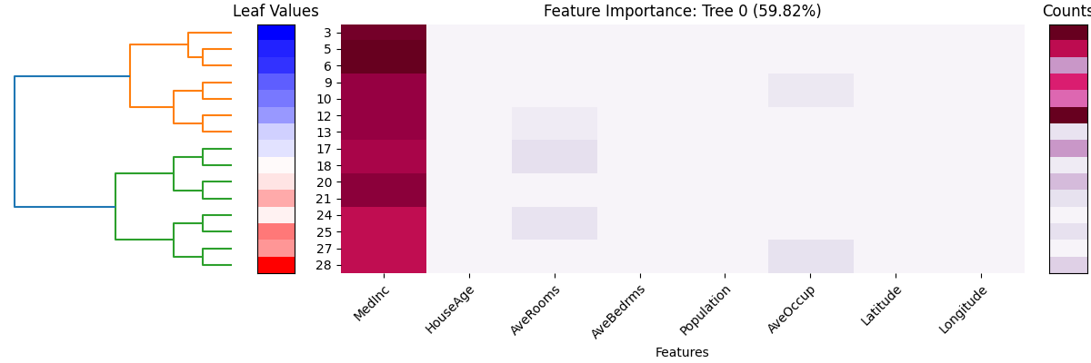
This plot is a summary of the leaf node information for the first tree in FIGS (tree_idx = 0). The title tells the importance of this tree, which is calculated by the normalized variance of \(\hat{f_{k}}\), using the training data. The x-axis represents the feature names, while the y-axis represents the leaf node ID. In the left column, the color scheme used represents the value of the leaf node. Blue shades are used for smaller values, while red shades are used for larger values. The hierarchical clustering dendrogram demonstrates how these leaf nodes are related to each other.

The subplot in the middle displays the importance (sum of gain) of each feature in the decision path of each leaf node. The importance of each feature is represented by a color scale, where darker colors indicate higher importance. Thus, the deeper the color, the more important the feature on the leaf node. For example, the feature MedInc is the most important feature in this tree, as it is multiple times in splitting the tree and also reduces the loss the most.

The rightmost subplot of the visualization displays the number of samples in each leaf node of the decision tree. This information is conveyed through a color scale, where darker colors represent a higher number of samples.

5.4.2.2. Tree Diagram

In addition to the feature importance heatmap, we can also globally interpret FIGS using tree diagrams. Unlike tree models, FIGS may consist of multiple trees, so it is necessary to specify which tree to display by using the tree_idx argument.

exp.model_interpret(model="FIGS", show="tree_global", tree_idx=0, root=0,
                    depth=3, original_scale=True, figsize=(16, 10))

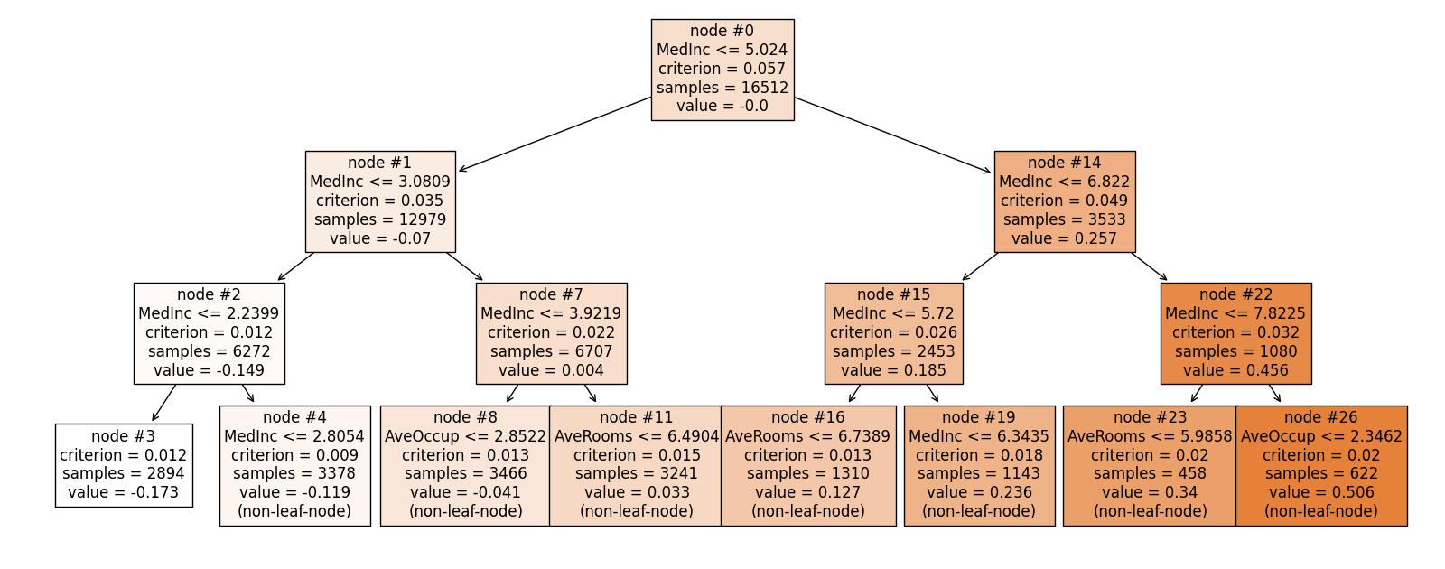
Here, the usage of root and depth is the same as that of Decision_Trees, which are used to control which part of the tree to display. The original_scale argument is used to control whether the feature values are scaled to the original scale. If original_scale is set to True, then the feature values are scaled to the original scale, otherwise, the feature values are by default scaled in the data preprocessing step. From this plot, it can be observed that MedInc is used multiple times to split the data. Furthermore, it is worth noting that in the root node, the average value is approximately zero, which is expected since the intercept term represents the overall mean of the response variable.

Next, we can also draw the diagram for the rest trees in FIGS. For instance, by setting tree_idx to 1, we can have the tree diagram for the second tree.

exp.model_interpret(model="FIGS", show="tree_global", tree_idx=1, root=0,
                    depth=3, original_scale=True, figsize=(16, 10))

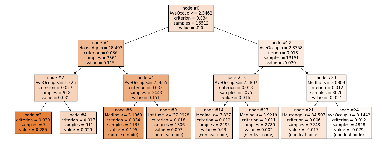
In this tree, AveOccup instead is the most important feature.

5.4.3. Local Interpretation

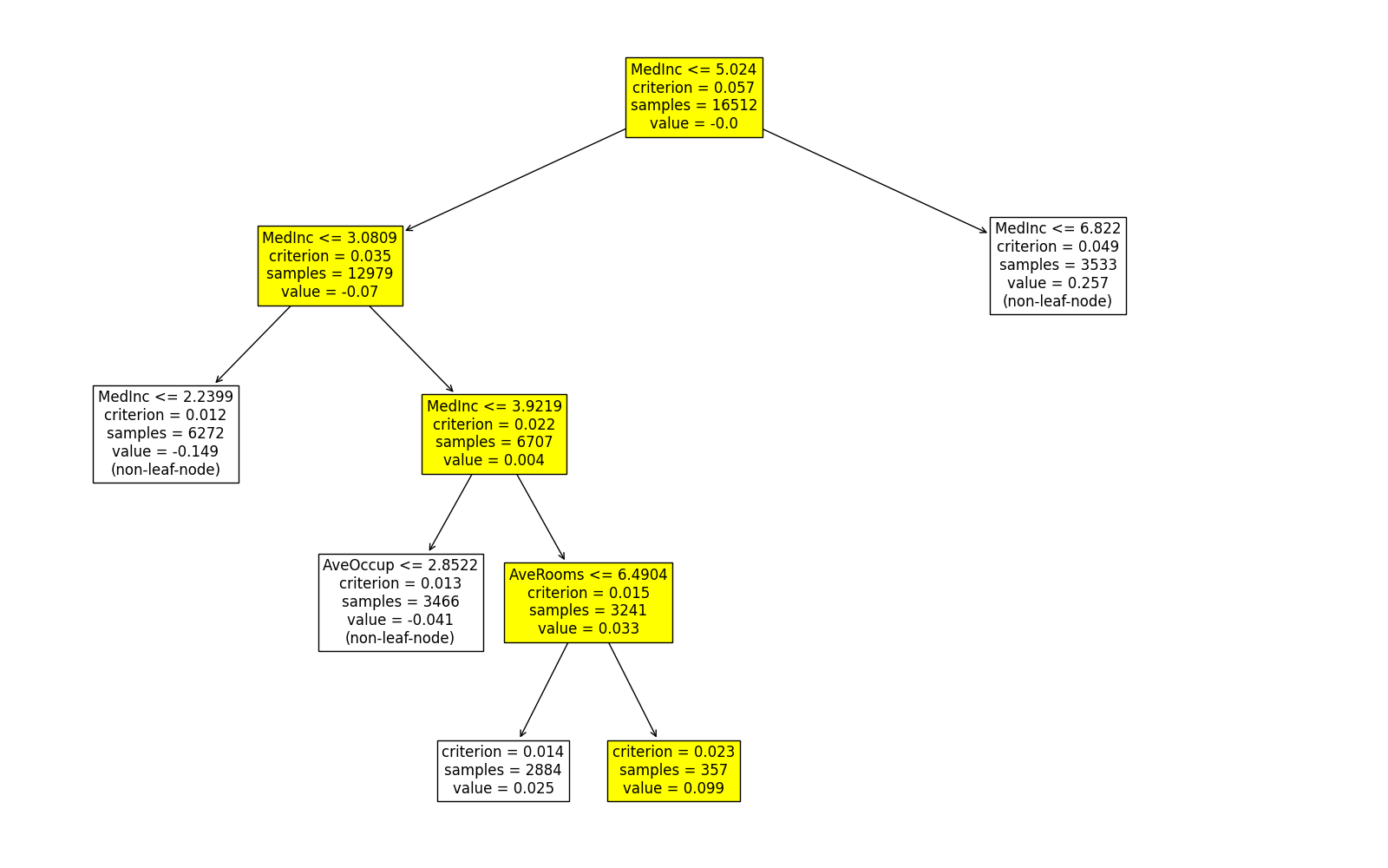
By using the “tree_local” keyword, the decision path of a chosen sample can be easily distinguished within the tree diagram. In addition, we need to specify the sample index to be interpreted in sample_id, as well as the tree_idx argument. The original_scale argument is also used to control whether the feature values are scaled to the original scale. For example, the following codes show the local interpretation of the first training sample on the first two trees.

exp.model_interpret(model="FIGS", show="tree_local", sample_id=0, tree_idx=0,
                    original_scale=True, figsize=(16, 10))

exp.model_interpret(model="FIGS", show="tree_local", sample_id=0, tree_idx=1,
                    original_scale=True, figsize=(16, 10))

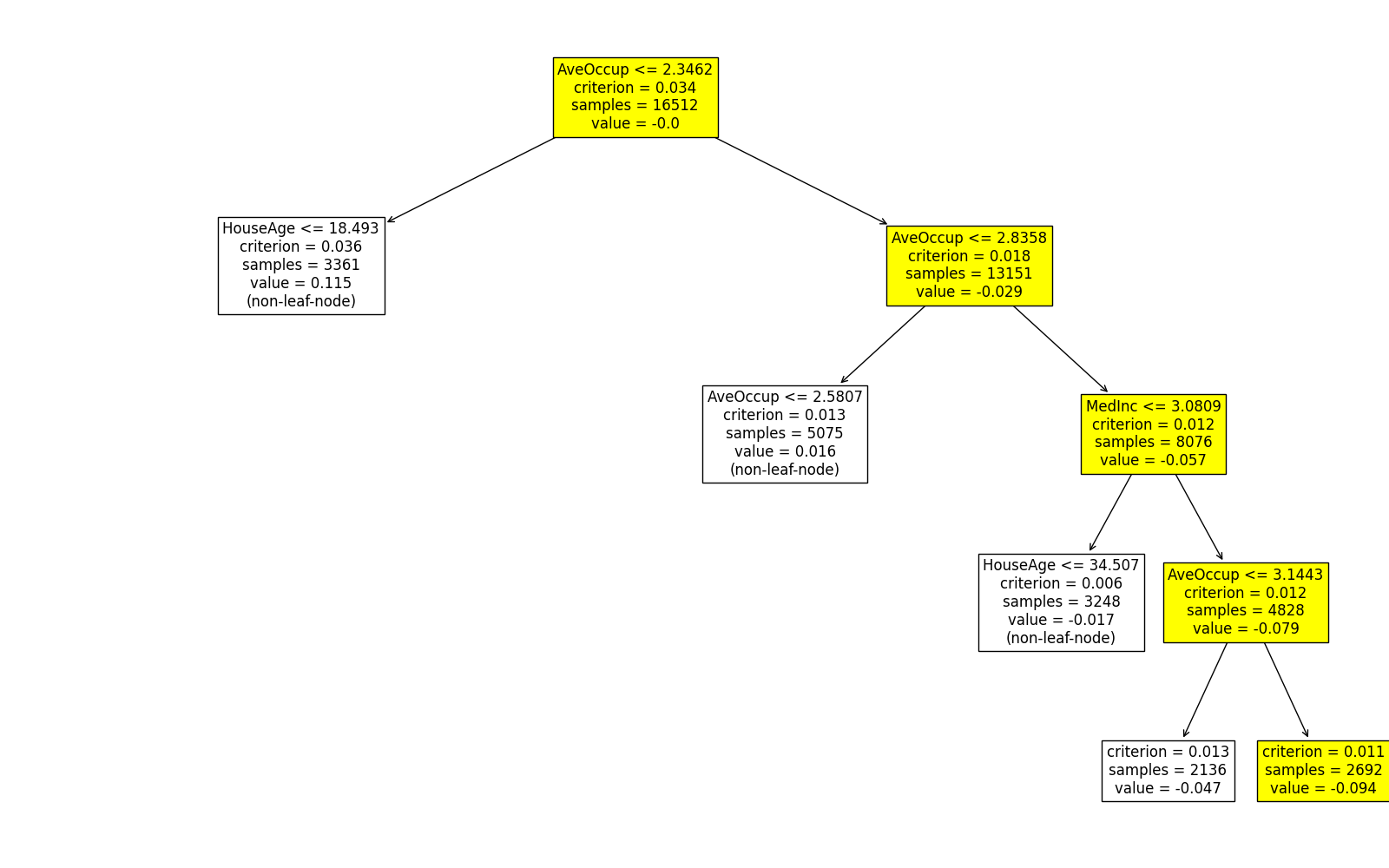
The predicted values of this sample on the first two trees are 0.099 and -0.094, respectively. Similarly, we can use the same approach to get the local interpretation of the first sample on the rest trees.

5.4.4. Examples

Example 1: CaliforniaHousing

The example below demonstrates how to use PiML with its high-code APis for the California Housing dataset from the UCI repository, which consists of 20,640 samples and 9 features, fetched by sklearn.datasets. The response variable MedHouseVal (Median Home Value) is continuous and is a regression problem.

• FIGS Regression (California Housing)

Examples 2: Taiwan Credit

The second example below demonstrates how to use PiML’s high-code APIs for the TaiwanCredit dataset from the UCI repository. This dataset comprises the credit card details of 30,000 clients in Taiwan from April 2005 to September 2005, and more information can be found on the TaiwanCreditData website. The FlagDefault variable serves as the response for this classification problem.

• FIGS Classification (Taiwan Credit)