5.5. XGBoost Depth 1

XGBoost depth 1 (XGB1) is a tree-based model that is suitable for both regression and classification problems. It is a special variant of XGB that restricts the maximum depth of the tree to 1, which is also referred to as boosted stumps [Lengerich2020]. XGB1 is interpretable since it can be interpreted as a GAM with piecewise constant main effects, as follows,

\[\begin{align} g(\mathbb{E}(y|\textbf{x})) = \mu + \sum\limits_{j} h_{j}(x_{j}), \tag{1} \end{align}\]

where \(\mu\) is the global intercept, \(h_{j}(x_{j})\) is the main effect of the \(j\)-th feature, and \(x_{j}\) is the \(j\)-th feature. The model is derived in the following steps.

Stage 1: Initial Model Fitting. In the first step, we fit an XGB model with a maximum depth of 1. The resulting model can be interpreted as a GAM with piecewise constant main effects, with the following procedures.

• Collecting the unique splits for each feature.

• Calculating the accumulated leaf node values for each bin generated by the unique splits.

The key feature of XGB1 is that it selects split points adaptively. This allows the model to achieve better predictive performance compared to spline-based GAMs, while still being interpretable. In addition to the above steps, we also perform the following two steps to further improve interpretability and model performance.

Stage 2: Binning Optimization. To improve interpretability and simplify the shape functions of XGB1, we optimize the binning of each feature. Specifically, we start by using the split points obtained from the raw XGB fitting results as the initial binning points. We then apply the optbinning package, a Python package for optimal binning, to optimize the binning points. The optimization process is based on the weight of evidence (WOE) of the binning and several constraints, such as the minimum bin size and the maximum number of bins. This step enables us to obtain a more interpretable model with simpler and easier-to-understand shape functions.

Stage 3: Refit the GAM with Optimized Bins. The final step involves refitting the GAM with the optimized bins. We provide two options for this step:

• GLM with one-hot encoding: Firstly, we transform each feature using one-hot encoding based on the binning results. Next, we fit a GLM using the one-hot-encoded features and the response. Finally, we re-arrange the fitted GLM coefficients into GAM format. If monotonic constraints are specified, we use the constrained GLM instead.

• XGB with ordinal encoding: Firstly, we transform each feature using ordinal encoding based on the binning results. Next, we fit another XGB model on the ordinal-encoded features and the response. Finally, we re-arrange the fitted XGB leaf values into GAM format. If monotonic constraints are specified, we turn on the corresponding monotonic constraints in XGB.

In summary, the XGB1 model is a special variant of XGB that restricts the maximum depth of the tree to 1. It is interpretable since it can be interpreted as a GAM with piecewise constant main effects. The model can be made more interpretable by the monotonicity and sparsity constraints.

5.5.1. Model Training

We use the California Housing dataset to demonstrate the training of the XGB1 model using the PiML workflow. The following steps are taken to train a raw XGB1 and a monotonicity constrained XGB1:

from piml.models import XGB1Regressor
exp.model_train(model=XGB1Regressor(n_estimators=100, max_bin=20, min_bin_size=0.01), name="XGB1")
exp.model_train(model=XGB1Regressor(n_estimators=500, max_bin=20, min_bin_size=0.01,
                mono_increasing_list=("MedInc", )), name="Mono-XGB1")

The XGB1Regressor (as well as XGB1Classifier) is developed based on the xgboost Python package and hence it inherits some commonly used hyperparameters in XGB, e.g., n_estimators and eta. To switch between the two options for the refit step, we provide a hyperparameter called fit_method. Setting fit_method to “glm” will use the GLM + one hot encoding option, while setting it to “xgb” will use the XGB + ordinal encoding option. This allows you to choose the method that works best for your particular use case.

5.5.1.1. Monotonicity Constraints

XGB1 model also supports monotonicity constraints. However, instead of manually typing in 0, 1, or -1 to indicate the direction of monotonicity for each feature in XGB, you can directly specify the feature names with their desired monotonic constraints using the following arguments in the XGB1 model.

• mono_increasing_list: the monotonic increasing constraints.

• mono_decreasing_list: the monotonic decreasing constraints.

With exp.model_train, the feature names are automatically inferred from the data. However, if you are using the XGB1 model separately, you may need to specify the feature_names parameter to ensure that the feature names are correctly identified; otherwise, the feature names will be set to “X0”, “X1”, etc.

5.5.1.2. Sparsity via Binning Optimization

In addition to the hyperparameters for XGB, we also provide hyperparameters for the binning optimization step. For example, you can control the binning results using the following two hyperparameters:

• max_n_bins: This hyperparameter specifies the maximum number of bins allowed for each feature during the binning optimization process. Increasing this value can result in more flexible binning, but may also increase the risk of overfitting.

• min_bin_size: This hyperparameter specifies the minimum number of samples allowed in each bin during the binning optimization process. Increasing this value can result in more stable binning, but may also lead to information loss if there are too few samples in a bin.

By tuning these hyperparameters, you can optimize the binning results to strike a balance between model complexity and interpretability. Increasing the max_bin hyperparameter or decreasing the min_bin_size hyperparameter may improve the model performance, but it may also increase the difficulty of model interpretation. Finding the right balance between these hyperparameters can help ensure that the model is both accurate and interpretable.

5.5.2. Global Interpretation

Similar to a GAM, there are multiple options available for interpreting a fitted XGB1 model, including main effect plots and feature importance plots. Additionally, we also provide options for drawing the Weight of Evidence (WoE) and Information Value (IV), which can further aid in the interpretation of the model.

5.5.2.1. Main Effect Plot

This plot shows the estimated effect of each feature on the predicted response while controlling for the effects of other features in the model.

exp.model_interpret(model="XGB1", show="global_effect_plot", uni_feature="MedInc",
                    original_scale=True, figsize=(5, 4))

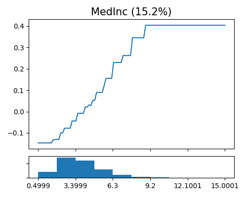
The above figure displays the estimated shape functions for the feature MedInc, accompanied by a histogram plot at the bottom. The estimated shape function appears to be piecewise constant, with an increasing trend for values of MedInc less than approximately 9.2, followed by a plateau. However, the estimated shape function is not strictly increasing, which is somehow inconsistent with commonsense.

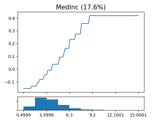
In comparison, the monotonicity constrained XGB1 model slightly sacrifices the predictive performance. But the correspondingly main effect of MedInc is strictly increasing, which makes it easy to interpret, as shown below.

exp.model_interpret(model="Mono-XGB1", show="global_effect_plot", uni_feature="MedInc",
                    original_scale=True, figsize=(5, 4))

5.5.2.2. Feature Importance

The keyword “global_fi” corresponds to the feature importance plot. Consistent with the rest additive models, the feature importance is calculated as the normalized variance of feature contributions, which gives us a measure of the relative importance of each feature in the model.

exp.model_interpret(model="Mono-XGB1", show="global_fi", figsize=(5, 4))

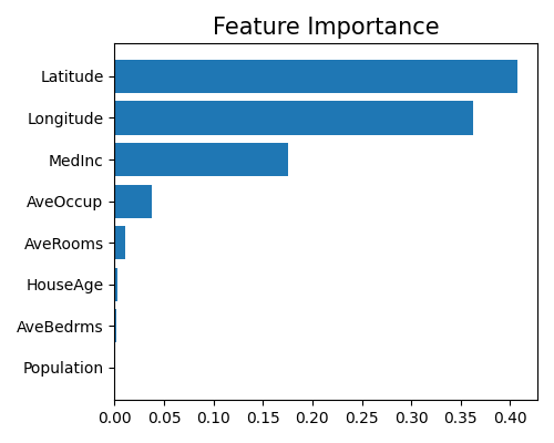
The two geographical features latitude and longitude are the most important features in the model, followed by MedInc and AveOccup. The feature Population is the least important in the model. Note that this plot only shows the top 10 features with the largest importance. To get the full results, you can set the parameter return_data to True.

5.5.2.3. Weight of Evidence Plot

The weight of evidence tells the predictive power of an independent variable in relation to the dependent variable. It is a measure of the strength of the relationship between the independent variable and the dependent variable. The WoE for a continuous target is computed as

\[\begin{align} \mathrm{WoE} = |U - \mu|, \end{align}\]

where \(U\) is the target mean value for each bin, \(\mu\) is the total target mean. The WoE for a binary target is computed as

\[\begin{align} \mathrm{WoE} = \log\frac{P(X|Y=0)}{P(X|Y=1)}. \end{align}\]

In PiML, you can draw the WoE plot of a given feature using the keyword “xgb1_woe” followed by the name of the univariate feature specified in uni_feature. The argument original_scale controls whether the feature values are displayed in the original scale or the transformed scale.

exp.model_interpret(model="Mono-XGB1", show="xgb1_woe", uni_feature="MedInc",
                   original_scale=True, figsize=(5, 4))

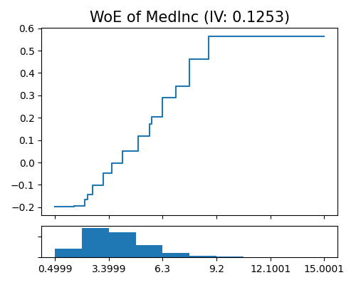
Comparing the WoE of MedInc to its main effect plot, it is evident that they are quite similar. However, the main effect plot has a smaller range compared to WoE. This is because WoE only displays the effect of MedInc on the target variable, while the main effect function factors in the impact of other features in the model, controlling for their effects while measuring the effect of MedInc on the target variable.

5.5.2.4. Information Value Plot

The information value is a valuable technique for selecting important variables in a predictive model by ranking them according to their importance. For a continuous target, the IV is the weighted average of WoE, which takes into account the sample size. For a binary target, the IV is also the weighted sum of WoE, as illustrated below.

\[\begin{align} \mathrm{IV} = \sum (P(X|Y=0) - P(X|Y=1)) \mathrm{WoE}, \end{align}\]

The code below shows the usage of drawing top-10 features IV with the keyword “xgb1_iv”.

exp.model_interpret(model="Mono-XGB1", show="xgb1_iv", figsize=(5, 4))

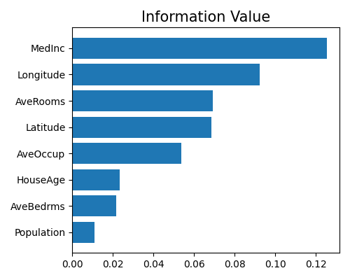
It turns out that the rank ordering of the IV plot is different from that of the feature importance plot. The feature MedInc is ranked as the most important feature in IV, followed by latitude, AveRooms, and longitude. The feature Population is still ranked as the least important feature. As latitude and longitude are highly correlated, the model may amplify the effect of latitude and longitude, which explains why they are ranked as the most important features in the feature importance plot. In contrast, the IV plot shows that MedInc is the most important feature, since the IV plot only considers the effect of each feature on the target variable. Note that this plot only shows the top 10 features with the largest information value. To get the full results, you can set the parameter return_data to True.

5.5.3. Local Interpretation

The local interpretation can be triggered by the keyword “local_fi”.

exp.model_interpret(model="Mono-XGB1", show="local_fi", sample_id=0, original_scale=True, figsize=(5, 4))

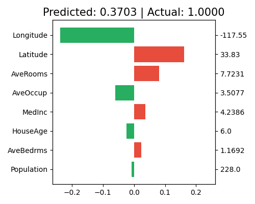
The title shows the actual response value and the predicted value of the chosen sample. Each bar in the plot represents the estimated effect value \(\hat{f}_j(x)\) of the chosen sample, which is the additive decomposition of the prediction. The right axis shows the feature values of the chosen sample. The feature Lontitude has the largest negative effect on the prediction, followed by Latitude and AveRooms. The feature Population has the least effect on the prediction. Note that this plot only shows the top 10 features with the largest contribution. To get the full results, you can set the parameter return_data to True.

5.5.4. Examples

Example 1: BikeSharing

The first example below demonstrates how to use PiML with its high-code APIs for developing machine learning models for the BikeSharing data from the UCI repository, which consists of 17,389 samples of hourly counts of rental bikes in Capital bikeshare system; see details. The response cnt (hourly bike rental counts) is continuous and it is a regression problem.

• XGB-1 Regression (California Housing)

Example 2: CoCircles

The example below demonstrates how to use PiML with the CoCircles data, which is a simulated binary classification data with two features exactly follow the GAM assumptions.

• XGB-1 Classification (CoCircles)