5.1. Generalized Linear Models

Generalized linear models (GLMs) are well known in the statistical literature and are among the most interpretable models. Readers should consult [McCullagh1989] for details.

GLMs are based on the assumption that, after a suitable transformation of the expected response, it has a linear relationship with the \(d\)-dimensional features \(x\). More specifically, the relationship is of the following form,

\[\begin{align} g(\mathbb{E}(y|\textbf{x})) = \mu + w_1 x_1 + w_2 x_2 + \ldots + w_d x_d, \tag{1} \end{align}\]

where \(\mu\) is the intercept term, \(w_1, w_2, \ldots, w_d\) are model coefficients (also called weights), and \(g(\cdot)\) is the link function. GLMs can be used to analyze continuous responses as well as binary, categorical, and count responses. The most popular link functions are the identity function \(g(x)=x\) for continuous responses, and the logit function \(g(x)=\log(x/(1-x))\) for binary responses.

5.1.1. Model Training

There are many existing packages for fitting GLMs under various settings and options. PiML integrates the scikit-learn implementations into GLMRegressor and GLMClassifier, with L1 and L2 regularization options.

• l1_regularization: The regularization strength of the L1 penalty, which penalizes the absolute values of model coefficients.

• l2_regularization: The regularization strength of the L2 penalty, which penalizes the squared values of model coefficients.

Both of these two regularization shrink the regression coefficients toward zero. With large L1 regularization, the fitted coefficients would become sparse. In contrast, with large L2 regularization, the fitted coefficients will be shrunk towards zero. The different combinations of these two hyperparameters would lead to different variants of GLMs.

GLMRegressor calls the following modules of scikit-learn.

• sklearn.linear_model.LinearRegression: Linear regression without constraint (l1_regularization=0, and l2_regularization=0).

• sklearn.linear_model.Lasso: Linear regression with L1 regularizer (l1_regularization>0, and l2_regularization=0).

• sklearn.linear_model.Ridge: Linear regression with L2 regularizer (l1_regularization=0, and l2_regularization>0).

• sklearn.linear_model.ElasticNet: Linear regression with elastic net regularizer (l1_regularization>0, and l2_regularization>0).

For binary regression (called classification in the ML literature), GLMClassifier directly uses the LogisticRegression class of scikit-learn.

• sklearn.linear_model.LogisticRegression: Logistic regression classifier with both L1 and L2 regularizer.

The following codes can be used to do model training.

from piml.models import GLMRegressor
exp.model_train(model=GLMRegressor(l1_regularization=0.0008, l2_regularization=0.0008), name="GLM")

We can test its performance using the model_diagnose function.

exp.model_diagnose(model="GLM", show="accuracy_table")

Using this command, a table would be generated, showing model performance on both train and test sets.

5.1.2. Global Interpretation

The exp.model_interpret function provides the capability to interpret a fitted model.

5.1.2.1. Regression Coefficients

In linear models, the regression coefficients estimate the change in the response variable for a unit change in the corresponding predictor variable, holding all other variables constant. This interpretation has to be adapted suitably for other link functions used in the GLM. For example,

• In a logistic regression model with a logit link function, the regression coefficient represents the change in the log odds of the response variable for a one-unit increase in the predictor variable.

When the predictor variables are measured on different scales, the coefficients cannot be directly compared. To address this issue, we standardize the predictor variables so that we can compare the coefficients on a comparable scale.

In PiML, we use the following command to show the regression coefficients of a fitted GLM, with the keyword “glm_coef_plot”.

exp.model_interpret(model="GLM", show="glm_coef_plot", figsize=(5, 4))

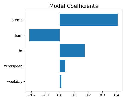
This plot shows the coefficients of the top 10 numerical features in a linear regression model, ranked by their absolute magnitude. A positive coefficient indicates that an increase in the corresponding feature value is associated with an increase in the response variable, while a negative coefficient indicates the opposite.

In this case, the plot suggests that the most important numerical feature in the model is temp (temperature), with a positive effect on the response variable. This is followed by hum (humidity), which has a negative effect on the response variable, and hr (hour), which has a positive effect on the response variable.

It is important to note that, in GLM, categorical variables are preprocessed by one-hot encoding, which involves converting each categorical variable into a set of binary variables representing each possible category. To visualize the coefficients of the categorical variables, a bar chart coefficient plot can be used. This involves plotting the coefficients for each category of the categorical variable separately, using the uni_feature parameter to specify the name of the categorical variable.

exp.model_interpret(model="GLM", show="glm_coef_plot", uni_feature="season", figsize=(5, 4))

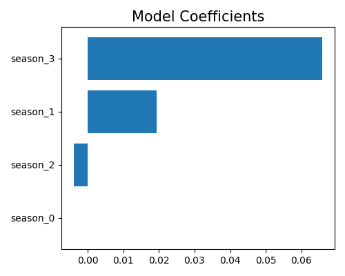
In this example, the categorical variable season has four categories, which are represented by four binary dummy variables: season_1, season_2, season_3, and season_4. To avoid overparameterization, only three of the four dummy variables are used for model fitting, and the fourth one (season_1) is dropped and assigned a coefficient of zero. Note that the choice of which dummy variable to drop can affect the interpretation of the coefficients for the remaining variables, especially if there are interactions or nonlinear effects between categories.

To get the results of all features, you can use the keyword “glm_coef_table”, and a data frame containing all features’ importance will be displayed. Instead of printing the table to the screen, you can also export the results to a data object by setting return_data to True.

exp.model_interpret(model="GLM", show="glm_coef_table")

5.1.2.2. Feature Importance

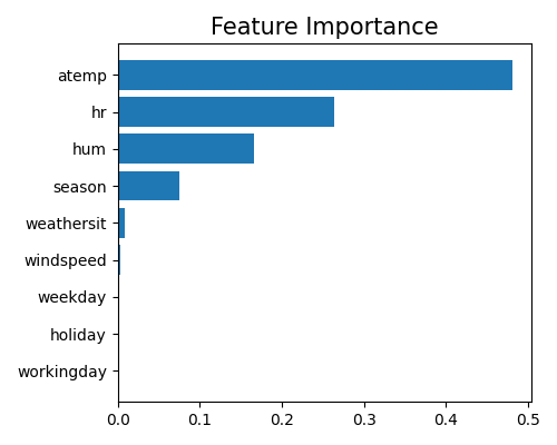
The feature importance measures the relative importance of each input feature in predicting the response. Here, the importance of each feature is calculated by measuring the variance of the marginal effect \(w_j x_j, (j = 1,\ldots,d)\) on the training set. For each categorical feature, we aggregate the marginal effects of all of its dummy variables and then calculate the variance. Therefore, the feature importance provides a measure of how much the feature contributes to the overall variability in the model’s predictions. In PiML, we use the keyword “global_fi” to trigger the feature importance plot.

exp.model_interpret(model="GLM", show="global_fi", figsize=(5, 4))

In order to interpret the relative importance of each feature as a proportion of the total importance across all features, we normalize the feature importance so that their sum equals 1. Because there may be many input features in a machine learning model, it can be helpful to focus on the most important features for interpretation and visualization purposes. Therefore, the feature importance plot typically shows only the top 10 most important features, to help identify which features are most relevant for understanding the model’s behavior and making predictions. To get the full results, you can set the parameter return_data to True.

5.1.3. Local Interpretation

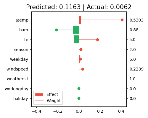
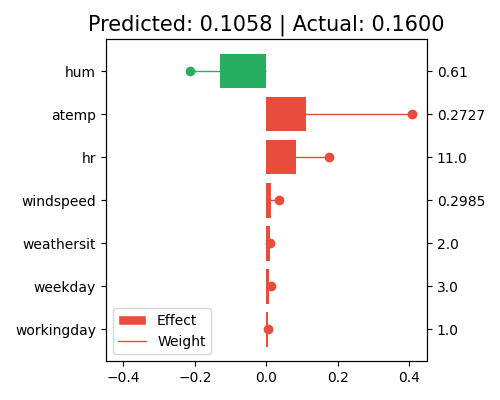
Local interpretation refers to the local contribution of each feature for a particular prediction on a single sample. In PiML, we can generate the local interpretation plot by keyword “local_fi”, together with the sample id to be interpreted, as follows.

exp.model_interpret(model="GLM", show="local_fi", sample_id=0, centered=False, original_scale=False, figsize=(5, 4))

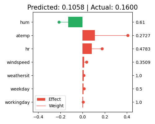
In this plot, the bars show the marginal contribution (effects) of each feature. The longer the bar, the larger the marginal effect, and the more contribution the corresponding feature has on the prediction. In contrast, the regression coefficients (weights) indicate the strength and direction of the relationship between each feature and the target variable. The larger the coefficient, the more sensitive the corresponding feature’ contribution to the prediction.

The sample_id=0 indicates that the plot is showing the marginal effects for the first sample in the training set, and the feature values for this sample are shown on the right axis. Note that this plot only shows the top 10 features with the largest contributions. To get the full results, you can set the parameter return_data to True.

5.1.3.1. Original Scale Option

The right axis of the local interpretation plot shows the scaled feature values. If you want to know the original feature values before the preprocessing, set original_scale=True.

exp.model_interpret(model="GLM", show="local_fi", sample_id=0, centered=False, original_scale=True, figsize=(5, 4))

5.1.3.2. Centered Option

In GLM, the interpretation of the marginal effects can be subject to model identifiability issues, where the marginal effect of a feature can be directly absorbed into the intercept term without changing the overall model prediction. This can result in unstable or arbitrary interpretations of the marginal effects.

To address this issue, a common approach is to center the features by subtracting the mean value of the feature from each observation. This can help to remove the identifiability problem and provide more stable interpretations of the marginal effects. In PiML, we set centered=True to turn on the centering option, as follows.

exp.model_interpret(model="GLM", show="local_fi", sample_id=0, centered=True, original_scale=True, figsize=(5, 4))

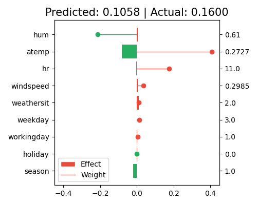
By centering the data and calculating the marginal effects, the model itself remains unchanged, but the interpretation of the marginal effects may change significantly, as we are essentially comparing the contribution of each feature to the average population, rather than the individual sample values. For instance, hum has a large contribution to the prediction in the uncentered data. However, when the data is centered, its contribution becomes negligible. This is because the feature value of this sample is close to the population mean, and its contribution is now mainly captured by the intercept term.

5.1.4. Data Dependent Interpretation

The model interpretation can be affected by the data distribution. For example, the feature importance of a feature can be very different for different data sets. To address this issue, we can use the use_test parameter to switch between training and testing data for interpretation. For example, the following command shows the feature importance of the GLM model on the testing data.

exp.model_interpret(model="GLM", show="global_fi", use_test=True, figsize=(5, 4))

For local interpretation, the sample_id parameter is used to select the sample in the training set. If you would like to interpret samples in the testing set, just set use_test to True. Then, the sample_id stands for the index of test set data.

exp.model_interpret(model="GLM", show="local_fi", sample_id=0, use_test=True,
                    original_scale=True, figsize=(5, 4))

5.1.5. Examples

Example 1: Bike Sharing

The first example below demonstrates how to use PiML with its high-code APIs for developing machine learning models for the BikeSharing data from the UCI repository, which consists of 17,389 samples of hourly counts of rental bikes in Capital bikeshare system; see details. The response cnt (hourly bike rental counts) is continuous and it is a regression problem.

• GLM Linear Regression (Bike Sharing)

Example 2: Taiwan Credit

The second example below demonstrates how to use PiML’s high-code APIs for the TaiwanCredit dataset from the UCI repository. This dataset comprises the credit card details of 30,000 clients in Taiwan from April 2005 to September 2005, and more information can be found on the TaiwanCreditData website. The data can be loaded directly into PiML, although it requires some preprocessing. The FlagDefault variable serves as the response for this classification problem.

• GLM Logistic Regression (Taiwan Credit)

References

[McCullagh1989]

Peter McCullagh, John Nelder (1989). Generalized linear models, Chapman and Hall - second edition.