5.2. Generalized Additive Model
In a generalized additive model (GAM), the primary effect of each feature is modeled using a non-parametric function, which can be expressed as:
In this equation, \(f\) represents the shape function, which is an unknown, smooth transformation of the features. This function can be estimated using a variety of methods, including smoothing splines, ensemble trees, or neural networks. Compared to GLM, the use of shape functions in GAMs allows for a more flexible and predictive model, as smooth functions can capture non-linear patterns in the data. However, to ensure model identifiability, the output of each shape function is assumed to have a zero mean.
5.2.1. Model Training
We demonstrate how to train a GAM using the CaliforniaHousing dataset and assume that this data has been well prepared. Next, we import the corresponding estimators, i.e., GAMRegressor or GAMClassifier, both based on the Python package pygam. As it is a regression problem, we use the GAMRegressor object with some customized hyperparameter settings.
from piml.models import GAMRegressor
exp.model_train(model=GAMRegressor(spline_order=1, n_splines=20, lam=0.6), name="GAM")
Below we briefly introduce some of its key hyperparameters.
spline_order: The degree of the piecewise polynomial representation.order 0: piecewise constant spline
order 1: piecewise linear spline
order 2: piecewise quadratic spline
order 3: piecewise cubic spline
n_splines: The number of knots in spline transformation refers to the number of anchor points used in estimating the shape function. With a larger number of knots, the estimated shape function tends to be more complex and able to capture more intricate patterns in the data. However, a higher number of knots also leads to a less smooth estimated function, which may result in overfitting the training data and poorer generalization to new data.lam: The regularization strength hyperparameter that controls the smoothness of the estimated shape function. This penalty term helps to prevent overfitting of the training data and encourages the model to learn simpler and more generalizable patterns in the data. By increasing the value oflam, the estimated shape function becomes smoother, which can capture more general patterns in the data. However, a smoother shape function may also result in a less predictive model. Conversely, a lower value oflamleads to a rougher shape function, which can capture more intricate patterns in the data, potentially resulting in overfitting.
5.2.2. Global Interpretation
For a fitted GAM, there are two common ways to interpret it globally, i.e., main effect plot and feature importance.
5.2.2.1. Main Effect Plot
This plot shows the estimated effect of each feature on the predicted response while controlling for the effects of other features in the model.
In GLM, the effect of each feature is a linear function, and the slope is determined by the regression coefficient.
In GAM, the effect of each feature can be of any shape, and this plot can be used to identify non-linear relationships between the features and the response and to assess the strength and direction of the relationship.
Below we show how to generate the global effect plot for GAMs, using the keyword “global_effect_plot”.
exp.model_interpret(model="GAM", show="global_effect_plot", uni_feature="MedInc",
                    original_scale=True, figsize=(5, 4))

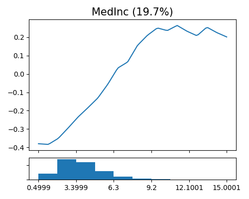
The figure above shows the estimated shape functions for the feature MedInc, together with the histogram plot on the bottom. It can be observed that the estimated shape function is piecewise linear as the order of spline is set to 1. The estimated shape function is relatively flat for the large values of MedInc, while we observe a steep increase in the beginning. This suggests that the median house price is relatively stable for most values of MedInc, but there is a sharp increase in median house price for low values of MedInc (less than 9.2). This indicates that MedInc is an important predictor for predicting the median house price, especially for low-income areas.
5.2.2.2. Feature Importance
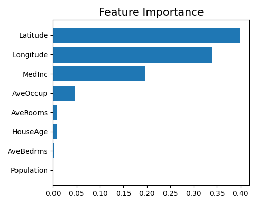
The keyword “global_fi” corresponds to the feature importance plot. The importance of the \(j\)-th feature is calculated by the variance of \(\hat{f}_j(x)\) using the training data. The feature importance is always non-negative and we also normalize them so that their sum equals 1.
exp.model_interpret(model="GAM",show="global_fi", figsize=(5, 4))

Due to space limitations, we display only the top 10 important features. To get the results of all features, you can manually set return_data=True, and then a data frame containing all features’ importance will be returned. From the plot above, we can see that the most important features are Latitude and Longitude, followed by MedInc and AveOccup.
5.2.3. Local Interpretation
This plot is useful for understanding how the model makes predictions for a particular data point and which features have the strongest influence on the prediction. It can also help identify the features that are driving the prediction. Similar to GLM, we use “local_fi” as the keyword for GAM’s local interpretation.
exp.model_interpret(model="GAM",show="local_fi", sample_id=0, original_scale=True, figsize=(5, 4))

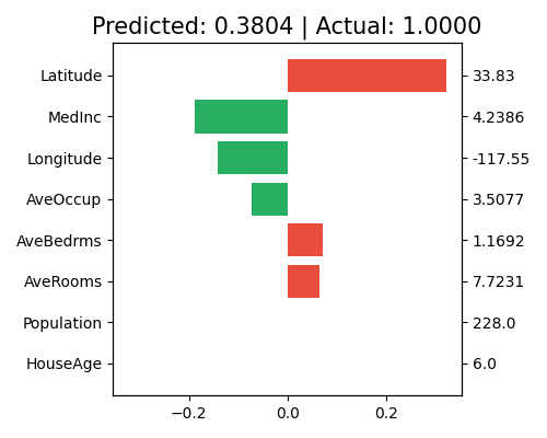
In this plot, the predicted value is 0.3804, while the actual response is 1.0. The bars represent the estimated effect values \(\hat{f}_j(x)\) of the chosen sample. The feature Latitude shows the largest positive contribution to the final prediction, while MedInc, Longitude, and AveOccup all have negative contributions.
Note that this plot only shows the top 10 features with the largest contribution. To get the full results, you can set the parameter return_data to True.
