5.3. Decision Tree
Decision tree is a well-known algorithm that operates by recursively dividing the dataset into smaller subsets based on the most influential features that can accurately predict the response. As the algorithm splits the data, it forms a tree diagram, rendering it highly interpretable.
5.3.1. Model Training
Assuming that the data has been prepared, one imports the appropriate module, which is either TreeRegressor for regression tasks or TreeClassifier for binary classification tasks. Once the appropriate module is imported, the next step is to use the exp.model_train method to fit the model to the data.
from piml.models import TreeRegressor
exp.model_train(model=TreeRegressor(max_depth=6), name="Tree")
Note that TreeRegressor (TreeClassifier) is a wrapper of sklearn.tree.DecisionTreeRegressor (sklearn.tree.DecisionTreeRegressor) in sklearn, in which we provide additional interpretation functionalities. When using decision trees, max_depth is often considered the most crucial hyperparameter. This parameter is commonly used for controlling the model complexity. Shallow trees are easy to interpret, but their predictive power might be limited. Deep trees, in general, would have better predictive performance, but can also suffer from overfitting and low model interpretability.
5.3.2. Global Interpretation
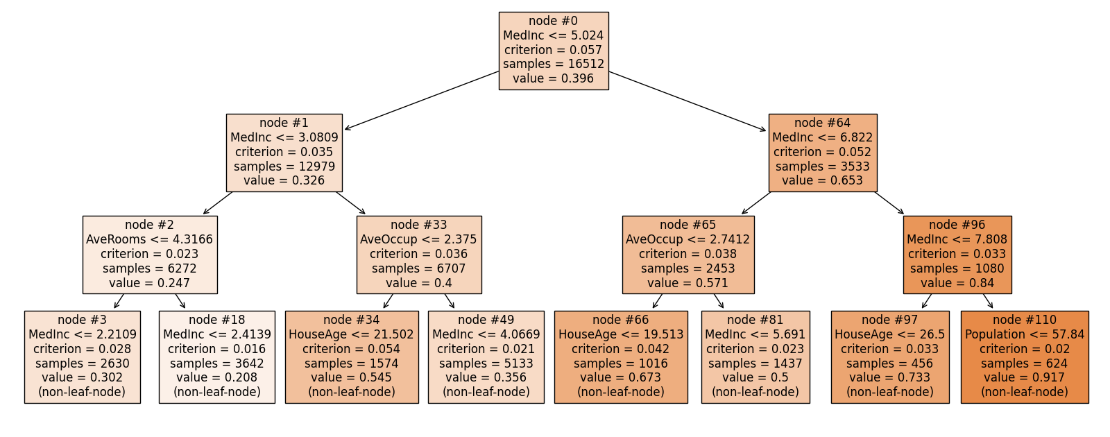
By setting show to “tree_global”, you will see the fitted decision tree diagram.
exp.model_interpret(model="Tree", show="tree_global", root=0,
                    depth=3, original_scale=True, figsize=(16, 10))

To ensure the tree diagram is useful for deep trees, we offer two parameters that enable you to adjust the view. The first is root, which is the node ID where the tree diagram begins. By default, it starts at the actual root node, which is assigned an ID of 0. The second parameter is depth, which sets the maximum depth of the diagram starting from the root node.
Each box in the diagram represents a node in the decision tree. It includes information such as the node ID, the splitting rule used to split the dataset, the criterion value, the sample size, and the average value of the response.
5.3.3. Local Interpretation
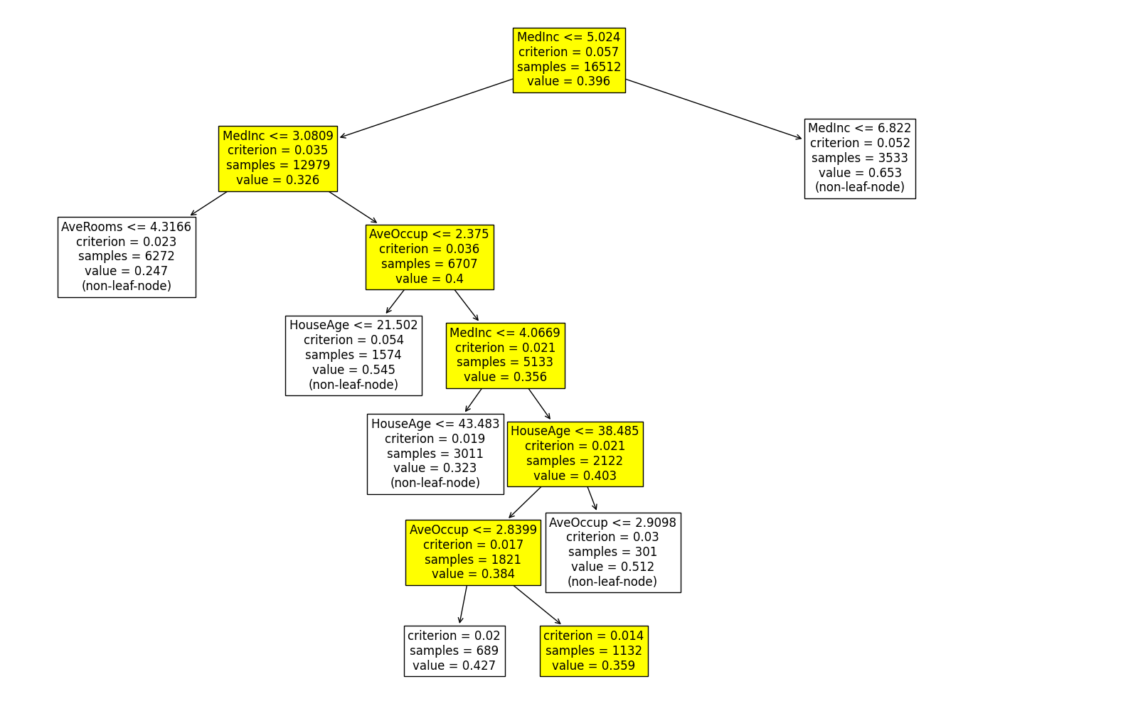
When using the “tree_Local” keyword, the decision path of a specific sample is highlighted within the tree diagram.
exp.model_interpret(model="Tree", show="tree_local", sample_id=0, original_scale=True, figsize=(16, 10))

Note that this plot may be a subset of the overall tree. Only the branches relevant to the selected sample are shown in the plot, making it easier to interpret the decision path of that particular sample within the context of the entire decision tree.
