6.3. Overfit

Overfitting is a prevalent issue in machine learning, characterized by a model’s strong performance on the training data but poor generalization to unseen or test data. Detecting overfitting is crucial as it enables model developers to take appropriate measures to prevent or alleviate its impact. Overfitting detection involves the identification of signs or patterns indicating that a model is overfitting to the training data. By recognizing these indicators, developers can gain insights into the model’s behavior and performance. This understanding empowers them to implement strategies such as regularization techniques, adjusting model complexity, or increasing the size of the training data to mitigate the overfitting problem and improve the model’s generalization ability.

6.3.1. Algorithm Details

Overfit detection shares similarities with weakspot detection but involves a slightly different approach. To evaluate the degree of overfitting of a fitted model, the following algorithm is employed:

• Run histogram binning of the 1 or 2 slicing features of interest.

• Calculate the train test performance gap within each bin.

The detection algorithm employed for overfit analysis is similar to that of weakspot detection. In the case of overfitting, we only provide the histogram slicing, which can effectively pinpoint overfit regions that highlight areas where the model exhibits prominent overfitting tendencies. This information enables model developers to take appropriate measures to address overfitting and enhance the model’s ability to generalize to unseen data.

6.3.2. Usage

To conduct an overfit assessment, you can use the model_diagnose function with the keyword “overfit” and the additional parameters listed below. Unlike the weakspot test, the overfit test does not require the use_test argument, as it is always performed on the test set.

• slice_method: This parameter allows you to choose the slicing method for the assessment. The only available option is “histogram” for now.

• slice_features: Specify the list of slicing features to be used. You should specify 1 or 2 slicing features; otherwise, a warning message will be displayed.

• bins: This parameter determines the number of bins for histogram slicing. The default value is set to 10.

• metric: Choose the performance metric for the assessment. The available options are “MSE” (default) and “MAE” for regression tasks, and “ACC” for classification tasks.

• threshold: Set the performance gap threshold ratio. The default value is 1.1, indicating a 10% increase above the average performance gap.

• min_samples: Specify the minimum sample size for considering a weak region. The default value is 20. Regions with a sample size below 20 will be ignored in the assessment.

By utilizing these parameters, you can perform an overfit assessment to identify regions where the model exhibits signs of overfitting based on the given slicing features and performance metrics.

6.3.2.1. One-way Overfit Plot

In the following demonstration, we will focus on a regression task using the BikeSharing data. Our goal is to identify overfit regions using the histogram method, with a particular emphasis on the variable hr.

results = exp.model_diagnose(model="XGB2", show="overfit", slice_method="histogram",
                             slice_features=["hr"], threshold=1.05, min_samples=100,
                             return_data=True, figsize=(5, 4))

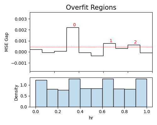
The analysis of overfit regions reveals that the most significant overfit region occurs when the variable hr is within the range of (7am, 9am). In this region, the test set exhibits a Mean Squared Error (MSE) of 0.0171, while the train set demonstrates an MSE of 0.0156. The observed gap between the test and train MSE is 0.0015, which exceeds the threshold value of approximately 0.0004, see the detailed information in the examples.

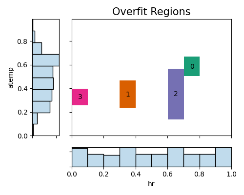
6.3.2.2. Two-way Overfit Plot

In the following analysis, we will identify overfit regions using histogram slicing with the variables hr and atemp. We have set the minimum sample size for considering a weak region to 100, ensuring that regions with an insufficient number of samples are not considered in the assessment. Additionally, the threshold ratio is set to 1.05, meaning that we consider regions with a performance gap greater than 1.05 times the average performance gap.

results=exp.model_diagnose(model="XGB2", show="overfit", slice_method="histogram",
                           slice_features=["hr", "atemp"], threshold=1.05, min_samples=100,
                           return_data=True, figsize=(5, 4))

6.3.3. Examples

Example 1: BikeSharing

The first example below demonstrates how to use PiML with its high-code APIs for developing machine learning models for the BikeSharing data from the UCI repository, which consists of 17,389 samples of hourly counts of rental bikes in Capital bikeshare system; see details. The response cnt (hourly bike rental counts) is continuous and it is a regression problem.

• Overfit: Regression

Examples 2: Taiwan Credit

The second example below demonstrates how to use PiML’s high-code APIs for the TaiwanCredit dataset from the UCI repository. This dataset comprises the credit card details of 30,000 clients in Taiwan from April 2005 to September 2005, and more information can be found on the TaiwanCreditData website. The data can be loaded directly into PiML, although it requires some preprocessing. The FlagDefault variable serves as the response for this classification problem.

• Overfit: Classification