6.7. Fairness

Fairness refers to the quality or state of being fair and impartial in the context of a model. When machine learning algorithms make decisions, it is essential to ensure that these decisions do not result in unfair outcomes based on sensitive variables. Examples of such variables include gender, ethnicity, sexual orientation, disability, and more. To address the issue of fairness, we introduce the model fairness test in this section. To illustrate the process, we provide example codes for initializing a PiML experiment using the Credit Simulation dataset. In the model training process, it is necessary to exclude demographic features such as “Race” and “Gender” from the training data to mitigate potential biases. We employ a monotonic depth 2 XGBoost algorithm to train the data, promoting fairness in the model’s decision-making process.

6.7.1. Fairness Metrics

PIML supports various fairness metrics, as shown below. In specific, we use the subscripts \(p\) and \(r\) to denote the protected and reference groups, respectively.

• AIR: Adverse impact ratio.

\[\begin{align} AIR = \frac{(TP_{p}+FP_{p}) / n_{p}}{(TP_{r}+FP_{r}) / n_{r}}. \end{align}\]

• Precision: Positive predictive value disparity ratio.

\[\begin{align} Precision Ratio = \frac{(TP_{p}) / (TP_{p}+FP_{p})}{(TP_{r}) / (TP_{r}+FP_{r})}. \end{align}\]

• Recall: True positive rate disparity ratio.

\[\begin{align} Recall Ratio = \frac{(TP_{p}) / (TP_{p}+FN_{p})}{(TP_{r}) / (TP_{r}+FN_{r})}. \end{align}\]

• SMD: Standardized mean difference between protected and reference groups. (Only used for regression tasks)

In PIML, you can use the model_fairness API to get the metric result, as follows,

metrics_result = exp.model_fairness(model="XGB2_monotonic", show="metrics", metric="AIR",
                group_category=["Race", "Gender"], reference_group=[1., 1.],
                protected_group=[0., 0.], favorable_threshold=0.5,
                figsize=(6, 4), return_data=True)

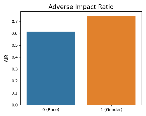
where “metrics” is the keyword for the parameter show. The metric parameter defines the fairness metric for evaluation. You also need to set the protected group and the reference group by the parameters group_category, reference_group, and protected_group. In the example above, we create two reference - protected group pairs:

• “Race” = 1.0 as reference and “Race” = 0.0 as protected;

• “Gender” = 1.0 as reference and “Gender” = 0.0 as protected;

The favorable_threshold parameter is the threshold for binarizing the predicted outcomes, usually set to 0.5 for binary classification. If return_data is true, the output results include:

• The plot of fairness metric result for each group.

• The detailed table of fairness metric results for each group.

6.7.2. Fairness Segmented

By leveraging the model_fairness API, we can also display fairness results conditioning on a feature of interest. The keyword of the parameter show is “segmented”, and the segmented feature can be specified by the parameter segment_feature.

• For numerical features, the desired number of equal-space bins can be controlled by the parameter segment_bins.

• For categorical features, the samples are segmented according to the unique categories present in the feature.

Once the segmentation is completed, PIML generates the fairness results for each bucket. The supported metric types align with those outlined in the “Fairness Metric” section. in PIML, users can effectively analyze and evaluate fairness at a granular level, allowing for a more comprehensive understanding of the model’s fairness performance across various segments of the data.

segmented_result = exp.model_fairness(model="XGB2_monotonic", show="segmented", metric="AIR",
                                       segment_feature="Balance", group_category=["Race","Gender"],
                                       reference_group=[1., 1.], protected_group=[0., 0.],
                                       segment_bins=5, favorable_threshold=0.5,
                                       return_data=True, figsize=(8, 4))

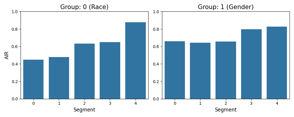
In this example, the segmentation feature is Balance and the number of bins is 5. If return_data is true, the following results would be returned:

• segmented_result.figure: The plot of segmented fairness metric results for each group.

• segmented_result.data: The detailed table of segmented fairness metric results for each group.

6.7.3. Fairness Binning

For unfair models, we provide two methods to mitigate the unfairness, where the model’s predictive performance may sacrifice. The first one is called feature binning, where we discretize / bin feature values that may lead to unfair results. There are three binning methods, quantile, uniform, and customize.

• Quantile binning: Assign the same number of observations to each bin.

• Uniform binning: Assign the same width in the span of possible values for the variable to each bin.

• Custom binning: Work for a specific area by replacing the original value with the mean value of this area.

The keyword for this strategy is “binning” for the show parameter. For quantile binning and uniform binning, PiML provides a grid search for the combination of bin numbers of multiple features. To configure the binning setting, you need to define the binning dictionary parameter binning_dict. Each binning setting is a key-value pair, see the example below. If binning type is “customize”, the value is the binning range, while if the type is “uniform” or “quantile”, the value is the number of bins. In addition to the fairness metric, the performance metric can also be specified by the parameter performance_metric.

binning_dict = {"Balance": {"type": "quantile", "value": [1, 5]},
                "Mortgage": {"type": "uniform", "value": [1, 5]},
                "Amount Past Due": {"type": "custom", "value": (0, 100)}}
binning_result = exp.model_fairness(model="XGB2_monotonic", show="binning", metric="AIR",
                                     group_category=["Race","Gender"],
                                     reference_group=[1., 1.], protected_group=[0., 0.],
                                     favorable_threshold=0.5, performance_metric="F1",
                                     binning_dict=binning_dict, return_data=True, figsize=(8,4))

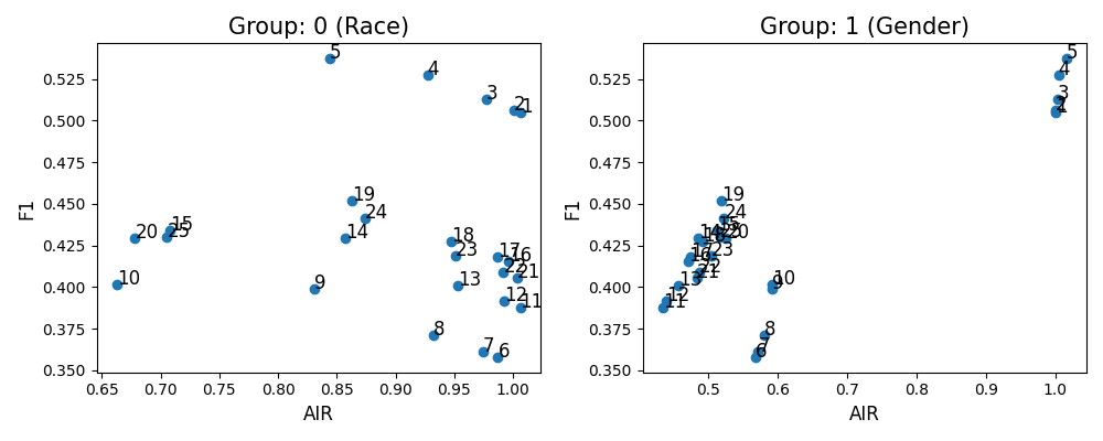
If return_data is true, the output results include:

• binning_result.figure: The plot of fairness and performance metric results with different binning settings.

• binning_result.data: The detailed table of fairness and performance metric results with different binning settings.

6.7.4. Fairness Thresholding

The second unfairness mitigation method is called thresholding, where we enumerate the classification threshold to get a better trade-off between fairness and performance. The keyword for this strategy is “thresholding” for the show parameter. In addition to the fairness metric, the performance metric can also be specified by the parameter performance_metric, and available metrics include “ACC” and “F1”.

thresholding_result = exp.model_fairness(model="XGB2_monotonic", show="thresholding", metric="AIR",
                                         group_category=["Race","Gender"],
                                         reference_group=[1., 1.], protected_group=[0., 0.],
                                         favorable_threshold=0.32, performance_metric="ACC",
                                         return_data=True)

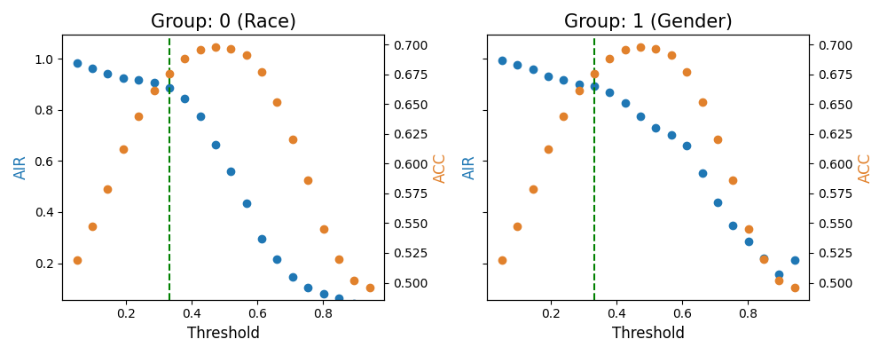
The favorable_threshold is the classification threshold value, which controls the dashed line position in the plots. The two y axes are controlled by metric and performance_metric, respectively. If return_data is true, the output results include:

• thresholding_result.figure: The plot of the fairness metric and performance metric results with a different threshold for each group.

• thresholding_result.figure: The detailed table of fairness metric and performance metric results with a different threshold for each group.

6.7.5. Examples

The full example codes of this section can be found in the following link.

Example

• Fairness Test: XGB2