6.8. Segmented

Segmented test is a separate model diagnostic module that is designed to diagnose the performance of a model in different segments. It is a powerful tool that can help users identify the weak regions of a model and provide insights into the root causes of the underperformance. In PiML, it can be triggered by the exp.segmented_diagnose function.

6.8.1. Methodology

Once a model is fitted and registered in PiML, this test facilitates a detailed evaluation of model weaknesses. It begins by segmenting the data into distinct subsets based on a selected feature of interest, followed by individual analyses for each subset. Notably, three segmentation methods are available:

• ‘uniform’: Segmentation based on equal intervals.

• ‘quantile’: Segmentation based on equal quantiles.

• ‘auto’: Automatic segmentation of feature segments determined by a surrogate model. The process involves fitting an XGB1 model between covariates and the residual, extracting split points from the XGB1 model, and using these points to segment the data. It’s important to note that some features may have no split points.

6.8.2. Usage

The exp.segmented_diagnose function has the following arguments.

• show: The available test keywords include

  • ‘segment_table’: the accuracy of each segment. If segment_feature = None, the results for all features will be output.

  • ‘accuracy_residual’: the residual plot of the specified segment and feature of interest.

  • ‘accuracy_table’: the accuracy results of the specified segment.

  • ‘weakspot’: the weakspot test of the specified segment.

  • ‘distribution_shift’: the density plot comparison between the specified segment and its complement.

• segment_method: The segmentation method, including “uniform”, “quantile”, and “auto”.

• segment_bins: The number of bins, used when segment_method is “uniform” or “quantile”.

• segment_feature: Feature filter for bucketing, only works when show = “segment_table”.

• segment_id: The ID of the segment to diagnose.

• metric: The performance metric for evaluation, which includes “MSE”, “MAE”, and “R2” for regression tasks, and “ACC”, “AUC”, ‘LogLoss’, ‘Brier’ and “F1” for classification tasks. The default metric is “MSE” for regression and “ACC” for classification.

6.8.2.1. Segments summary

In the segmented diagnose module, you can start by obtaining a summary of the segments, by setting the parameter show to ‘segment_table’. This table provides a summary of all segments and helps users quickly identify any regions of interest. Additionally, if you define the segment_feature parameter, the table will be filtered to only show the feature-related results of the segments.

result = exp.segmented_diagnose(model='XGB2', show='segment_table',
                                segment_method='uniform', segment_bins=5, return_data=True)
result.data

	Segment ID	Feature	Segment	Size	MSE
0	0	hr	[0.6, 0.8)	735	0.018380
1	1	hr	[0.2, 0.4)	712	0.014116
2	2	hum	[0.0, 0.2)	15	0.013335
3	3	hum	[0.2, 0.4)	441	0.013161
4	4	atemp	[0.5909, 0.7878)	1026	0.012643
5	5	season	2.0	912	0.011245
6	6	windspeed	[0.7298, 0.9123]	12	0.011149
7	7	workingday	0.0	1131	0.010764
8	8	windspeed	[0.1825, 0.3649)	1598	0.010634
9	9	season	3.0	874	0.010363

The table displayed above presents the top 10 weakest segments. It consists of the following columns:

• Segment ID: The ID of each segment.

• Feature: The segmented feature.

• Segment: The segment range if it is a numerical feature, segment value if it is a categorical feature.

• Size: The number of samples contained within each segment.

• metric: The metric value corresponding to each segment.

6.8.2.2. Accuracy Table

Once you have specified a specific segment_id, you can further analyze the performance of that segment. By setting show to ‘accuracy_table’, an accuracy table will be presented. This table provides information and insights regarding the accuracy of the segment you have chosen. It can provide valuable metrics and metrics-based analysis to help you understand the performance of that segment. For more details about the metrics, you can see: test_accuracy.

result = exp.segmented_diagnose(model='XGB2', show='accuracy_table', segment_id=0, return_data=True)
result.data.head(10)

	MSE	MAE	R2
Train	0.0081	0.0692	0.8144
Test	0.0089	0.0721	0.8018
Gap	0.0008	0.0028	-0.0126

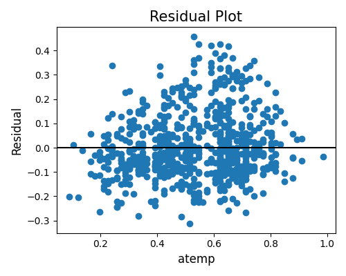
6.8.2.3. Residual Plot

The residual represents the distinction between the actual response values and the predicted response values, showcasing the variance between anticipated and observed outcomes. When the show parameter is configured as ‘accuracy_residual’, the corresponding residual plot will be generated. Nevertheless, to produce this plot, it is essential to define the show_feature parameter. This parameter is instrumental in pinpointing the particular feature or variable under analysis concerning the residuals. For a more comprehensive understanding of the residual plot, refer to the documentation on test_accuracy_residual.

exp.segmented_diagnose(model='XGB2', show='accuracy_residual', segment_id=0, show_feature='atemp')

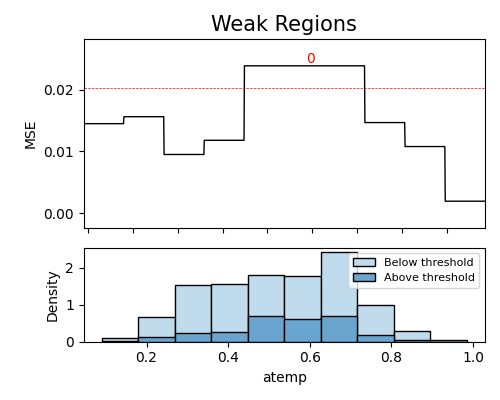
6.8.2.4. Weakspot

When show is set to ‘weakspot’, the weakspot test will be executed. Similar to the weakspot in the model diagnose module, there are several arguments that can be customized. These arguments include:

• slice_method: Specifies the method to slice the data for analysis.

• slice_features: Determines the features or variables to consider during the slicing process.

• bins: Defines the number of bins or intervals to divide the data into.

• metric: Refers to the evaluation metric used to measure the strength of the weak regions.

• threshold: Sets the threshold value for identifying weak regions.

• min_samples: Specifies the minimum number of samples required to consider a region as weak.

• use_test: Determines whether to use the test set for analysis.

By adjusting these arguments, you can customize the weakspot analysis to suit your specific needs. For more details about weakspot, you can find from test_weakspot.

exp.segmented_diagnose(model='XGB2', show='weakspot', segment_id=0, slice_features=['atemp'])

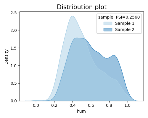
6.8.2.5. Distribution shift

After pinpointing a specific segment, it becomes crucial to comprehend the extent to which that segment differs from its complement, i.e., the data drift test with the keyword ‘distribution_shift’. The test introduces additional arguments:

• show_feature: This parameter can be employed to compare the marginal densities of the segment and its complement for a particular feature. If the show_feature parameter is undefined, the marginal distances for all features will be displayed.

• distance_metric: This parameter provides the flexibility to alter the distance metric shown on the plot. The default distance metric is PSI. It can also be set to “WD1” or “KS”.

• psi_buckets: Responsible for modifying the binning method during PSI (Population Stability Index) calculation. The default binning method is “uniform”, and it can be adjusted to “quantile”.

For more details, see: twosample_test.

exp.segmented_diagnose(model='XGB2', show='distribution_shift', segment_id=0)

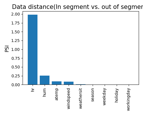
The presented plot offers valuable insights into disparities in feature distributions, offering clarity on the underlying reasons for underperformance within the segment. Moreover, the optional argument distance_metric provides the flexibility to choose the preferred distance metric for the analysis.

If the show_feature parameter is specified, the generated plot will center specifically on the distribution drift of the chosen feature, providing a more focused examination.

exp.segmented_diagnose(model='XGB2', show='distribution_shift', segment_id=0, show_feature='hum')

6.8.3. Examples

Example 1: BikeSharing

The first example below demonstrates how to use PiML with its high-code APIs for developing machine learning models for the BikeSharing data from the UCI repository, which consists of 17,389 samples of hourly counts of rental bikes in Capital bikeshare system; see details. The response cnt (hourly bike rental counts) is continuous and it is a regression problem.

• Segmented Diagnose (Regression)

Examples 2: SimuCredit

The second example below demonstrates how to use PiML’s high-code APIs for the SimuCredit dataset. The Approved variable serves as the response for this classification problem.

• Segmented Diagnose (Classification)