6.2. WeakSpot

Weakness detection involves identifying areas or regions where a model is prone to underperform or make incorrect predictions. These weaknesses can arise due to factors like inadequate or biased data, overfitting, the use of unsuitable algorithms, or insufficient model complexity. It is essential to identify and address these weaknesses to enhance the accuracy and reliability of the model. In PiML, the weakspot test allows us to identify weak regions in a fitted model using different slicing techniques. More details on this feature are provided below.

6.2.1. Algorithm Details

To conduct a weakspot test on a fitted model, the following steps are performed:

• Specify 1 or 2 slicing features: Choose one or two features that you want to use for segmenting the data.

• Segment the data: Apply an unsupervised or supervised binning technique to the selected slicing features.

• Evaluate performance metric: Calculate the performance metric of interest for each binning segment.

• Filter out weak regions: Apply filters based on performance thresholds and minimum sample constraints to identify weak regions. These filters help determine regions where the model’s performance falls below a certain threshold and where the number of samples is sufficient for reliable analysis.

By following these steps, you can effectively identify and analyze areas of weakness in the model’s predictions. Specifically, in PiML, there are three available slicing methods for detecting weak regions: histogram slicing and tree slicing.

• Histogram Slicing: This method utilizes unsupervised binning to partition the features of interest into equal-space bins. The number of bins defaults to 10. However, if the number of unique values is less than 10, these unique values are utilized as the split points. When two slicing features are specified, the process begins by conducting histogram binning on one feature. Subsequently, for each bin, histogram binning is performed on the second feature.

If connected bins are identified as weak regions, our approach involves merging them into a single bin. This merging process is relatively simple when dealing with only one slicing feature. However, when two slicing features are involved, we condition one dimension and merge the weak regions along the other dimension.

• Tree Slicing: This approach employs a supervised binning method. The initial step is to calculate a specific metric for each sample, such as square error for MSE, absolute error for MAE, or correct/incorrect status for accuracy score. Next, a decision tree model is fitted using the features of interest as predictors and the individual metrics as the response. The decision tree is configured with max_depth=3 and min_samples_leaf as the minimum sample size. The generated decision tree is then utilized to create bins, and the performance of each bin is assessed accordingly.

Note

The supervised binning method, i.e., tree slicing, is suitable for cases where the metric is additive. This means that the metric for the entire sample can be calculated by aggregating the metric values of individual samples. For instance, metrics such as “MSE” (Mean Squared Error), “MAE” (Mean Absolute Error), “ACC” (Accuracy Score), “LogLoss” (Log Loss), and “Brier” (Brier Score) are additive in nature. However, metrics like “R2” (R-squared), “AUC” (Area Under the Curve), and “F1” (F1 Score) are not additive. By default, the “MSE” metric is used for regression tasks, while “ACC” is used for classification tasks.

6.2.2. Usage

For demonstration purposes, we consider an XGB2 model on the TaiwanCredit data. Weakspot assessment can be conducted by employing the model_diagnose function. To evaluate weak regions, simply set the show parameter to “weakspot”. Moreover, the following parameters offer increased flexibility for customization and analysis.

• slice_method: This parameter allows you to select the desired slicing method from the available options: “histogram” and “tree”, which correspond to the three aforementioned slicing methods. The default value is “histogram”.

• slice_features: This argument is used to specify the list of slicing features. For weakspot analysis, you need to specify 1 or 2 slicing features; otherwise, a warning message will be displayed.

• bins: This parameter determines the number of bins used for histogram slicing. By default, it is set to 10.

• metric: You can choose the performance metric for evaluation, which includes “MSE”, “MAE”, and “R2” for regression tasks, and “ACC”, “AUC”, “F1”, “LogLoss”, and “Brier” for classification tasks. The default metric is “MSE” for regression and “ACC” for classification.

• threshold: This parameter represents the performance metric threshold ratio used to distinguish between weak and good regions. The default value is set to 1.1, which corresponds to a 10% performance drop compared to the average metric. For example, if the AUC of the entire sample (train or test set) is 0.8, then the threshold would be calculated as 0.8 / 1.1 = 0.723. Regions with an AUC value lower than 0.723 will be classified as candidate weak regions. However, for metrics like MSE in regression tasks, the threshold is computed as 0.8 * 1.1 = 0.88 (also assuming the MSE for the entire sample is 0.8), as a smaller MSE value is considered better. Consequently, regions with an MSE greater than 0.88 will be identified as weak regions.

• min_samples: This parameter sets the minimum sample size required for a region to be considered weak. The default value is 20. Regions with a sample size below 20 will be ignored during the assessment.

• use_test: This boolean parameter allows you to switch between using the training or testing data. By default, it is set to False, indicating the use of the training data. To utilize the testing data, you can set use_test to True.

6.2.2.1. One-way WeakSpot Plot

In the following demonstration, we will identify weak regions using the testing data (use_test=True). The chosen slice method is “histogram”, with a threshold ratio of 1.1. We will consider a minimum sample size of 100 for the weak regions analysis. Specifically, we will focus on a single slicing feature, PAY_1.

results = exp.model_diagnose(model="XGB2", show="weakspot", slice_method="histogram",
                        slice_features=["PAY_1"], threshold=1.1, min_samples=100, metric="ACC",
                        use_test=True, return_data=True, figsize=(5, 4))

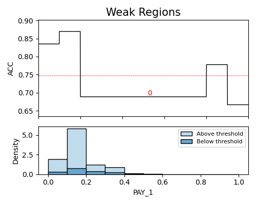
The above plot illustrates the detection of a single weak region for the feature PAY_1. The red dotted line represents the performance threshold, which is calculated by dividing the average metric (around 0.82) by the user-specified threshold ratio (1.1), resulting in a threshold value of approximately 0.75. Each weak region is annotated with its corresponding weak region number.

On the x-axis, we have the variable of interest (PAY_1), while the y-axis represents the density and accuracy score of each segment. In the density plot, the “Above threshold” and “Below threshold” labels indicate the population segments with prediction errors greater or less than the threshold, respectively. However, it is important to note that for metrics such as “AUC”, “F1” in classification tasks, or “R2” in regression tasks, which are not additive, the density plot does not display the “Above threshold” and “Below threshold” labels. The detailed information of detected weak regions can be found in the returned table, as we set return_data to True.

The table above shows the weak regions of the testing data. It contains the following columns:

• [feature_name: The lower bound of the slicing feature;

• feature_name): The upper bound of the slicing feature;

• #Test: The number of samples in the testing set;

• #Train: The number of samples in the training set;

• test_metric: The performance metric of the weak region on the testing set;

• train_metric: The performance metric of the weak region on the training set;

• Gap: The difference between the testing and the training performance metric.

Note that if no weak region is detected, then a message saying “No weak regions detected.” will be displayed, and the results object will become None. Note that as there exist multiple weak regions, the order of weak regions is determined by the gap between the testing and the training performance metrics.

Note that if no weak regions are detected, a message stating “No weak regions detected.” will be displayed, and the results object will be None. In cases where multiple weak regions are identified, the order of the weak regions is determined based on the gap between the performance metrics of the testing and training datasets.

It is important to note that the original_scale argument solely affects the plot visualization, allowing for the representation of data in its original scale. However, the table presented in the analysis retains the use of scaled values for consistency and accurate comparisons.

6.2.2.2. Two-way WeakSpot Plot

In the following demo, we identify weak regions of the testing data (use_test=True) using two slicing features, i.e., PAY_1 and PAY_2. We set the minimum sample size as 100 and use the histogram slicing.

results = exp.model_diagnose(model="XGB2", show="weakspot", slice_method="histogram",
                       slice_features=["PAY_1", "PAY_2"], threshold=1.1, min_samples=100, metric="ACC", use_test=True, return_data=True, figsize=(5, 4))

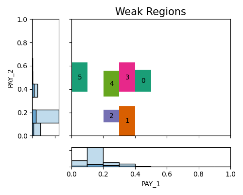
In this particular demonstration involving two variables, the plot reveals the presence of 5 weak regions. The accompanying summary table provides additional information regarding each region. It includes the testing and training accuracy scores for the samples within each region, as well as the gap between the testing and training ACC scores. These details offer insights into the performance discrepancy between the testing and training datasets for each specific region. Let’s take Region 0 as an example, which consists of 191 testing samples and 800 training samples. This region corresponds to the range of PAY_1 values between 2.6 and 3.5, and PAY_2 values between 2.2 and 3.6.

6.2.3. Examples

Example 1: BikeSharing

The first example below demonstrates how to use PiML with its high-code APIs for developing machine learning models for the BikeSharing data from the UCI repository, which consists of 17,389 samples of hourly counts of rental bikes in Capital bikeshare system; see details. The response cnt (hourly bike rental counts) is continuous and it is a regression problem.

• WeakSpot: Regression

Examples 2: Taiwan Credit

The second example below demonstrates how to use PiML’s high-code APIs for the TaiwanCredit dataset from the UCI repository. This dataset comprises the credit card details of 30,000 clients in Taiwan from April 2005 to September 2005, and more information can be found on the TaiwanCreditData website. The data can be loaded directly into PiML, although it requires some preprocessing. The FlagDefault variable serves as the response for this classification problem.

• WeakSpot: Classification