6.5. Robustness

The performance of a model can be adversely affected when it encounters noisy data or experiences distribution shifts. This can result in incorrect predictions. Such data drift or shift may occur due to unexpected changes, which can alter the underlying patterns and relationships between the input and target variables. In this section, we will demonstrate how to utilize PiML to evaluate the model’s robustness to input perturbations.

6.5.1. Algorithm Details

The robustness test assesses model performance to small changes in the covariate space. It proceeds as follows,

• Perturb \(x\) with changes \(\Delta x\).

• Calculate the model’s output \(\hat{f}(x + \Delta x)\) on perturbed data.

• Evaluate the performance metric of \(Score(y, \hat{f}(x + \Delta x))\).

This process is iterated ten times for all the test samples, with performance metrics recorded for each repetition. It is important to note that the assumption is made that the response remains unchanged throughout. Perturbation can be applied to both numerical and categorical features. The forthcoming sections will illustrate the perturbation methods for numerical and categorical features, respectively.

6.5.1.1. Perturbation For Numerical Features

For numerical features, we provide the following two perturbation options.

• Raw perturbation: Directly add i.i.d. Gaussian noise \(N(0, \lambda^2 var(x))\) to \(x\), where \(\lambda\) is the perturbation size (the argument perturb_size to be used in the model_diagnose function). However, this method may not be suitable when

  1. The data is discrete, e.g., 1, 2, 3, … 10. In this case, the perturbed data, e.g., 1.2 may become invalid.

  2. The data is skewed and has a long tail distribution. In this case, the calculation of standard deviation may become unstable, and it is relatively hard to choose a suitable perturbation size.

• Quantile Perturbation: Quantile perturbation can solve the above issues. First, the feature \(x\) is converted to the quantile space. The uniform noise \(U(-0.5 \lambda, 0.5 \lambda)\) is then added to perturb the quantiles. Here \(\lambda\) also represents the perturbation size. Finally, transform the quantiles to the original space. The following table demonstrates this process.

x	1	2	2	2	3	3	3	40	40	50
Quantile	0.1	0.2	0.3	0.4	0.5	0.6	0.7	0.8	0.9	1.0

Let’s take into account a data point with a value of 3, along with its corresponding quantile value of 0.7. On the quantile scale, a small noise of 0.12 is generated and added to the original quantile value of 0.7. This sum yields a resulting value of 0.82, which is then rounded to the nearest available value, namely 0.8. Finally, the perturbed quantile is transformed back to the original scale, resulting in a value of 40.

6.5.1.2. Perturbation for Categorical Variable

For illustration, let’s assume we have three categories (A, B, and C). First of all, we summarize the frequency of each category in the data, e.g., 30%, 30%, and 40%, respectively. Then, each sample is perturbed with probability \(p\) (perturb_size) and kept unchanged with probability \(1-p\). For example, if \(p=0.3\), then 30% of the samples will be perturbed. If a sample is perturbed, it will be perturbed to A, B, and C with probability 30%, 30%, and 40%, respectively.

6.5.2. Usage

To perform a robustness test using the model_diagnose function, you have two options: “robustness_perf” and “robustness_perf_worst”. The former evaluates the model’s robustness under perturbation overall testing samples, while the latter only assesses the model’s robustness on the worst test samples. The following arguments are required to run the robustness test:

• perturb_method: This parameter determines the perturbation method for numerical features. The default option is “raw”, which involves adding normal noise to the covariates for perturbation. Alternatively, you can choose “quantile”, which perturbs the data in the quantile scale.

• perturb_features: Specify the features to be perturbed. By default, this is set to None, which means all features will be perturbed. You can also provide a list of feature names if you only want to perturb selected features.

• perturb_size: This parameter represents the perturbation step or magnitude. It determines the amount of perturbation applied to the data.

• metric: Select the performance metric to be used for evaluation. Supported metrics depend on the type of task. For binary classification, the options are “ACC” (accuracy), “AUC” (Area Under the Curve), and “F1” (F1 score). For regression tasks, the options are “MSE” (Mean Squared Error), “MAE” (Mean Absolute Error), and “R2” (R-squared).

• alpha: This parameter specifies the proportion of worst samples to consider when evaluating the performance against perturbation sizes.

As an illustrative example, let’s consider a FIGS model applied to the BikeSharing dataset.

6.5.2.1. Robustness on the whole test sample

To assess the models’ performance against noise, we set the parameter show to “robustness_perf”.

exp.model_diagnose(model="FIGS", show='robustness_perf', perturb_features=None,
                  perturb_method="raw", metric="MSE", perturb_size=0.1, figsize=(6, 4))

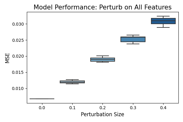
In the figure above, the x-axis represents the noise level, indicating the magnitude of perturbation applied to the data. The y-axis displays the test set performance of the model after perturbation. The box plot illustrates the results obtained from ten repetitions of the experiment. When the noise level is set to 0.0, there is no perturbation applied, resulting in no variation in the model’s performance. As the noise level increases, we observe a degradation in the model’s performance, which is expected. The full plot captures the model’s performance at each noise level, providing an overview of how the model’s performance changes with increasing perturbation.

In the second example, we will specifically perturb two features: hr and atemp. The remaining settings will be kept the same as in the first example. This means we will use the same perturbation method, perturbation step, and performance metric. By perturbing a smaller number of features, the observed degradation in model performance is expected to be smaller compared to the first example where all features were perturbed.

exp.model_diagnose(model="FIGS", show="robustness_perf", perturb_features=["hr", "atemp"],
                  perturb_method='raw', metric="MSE", perturb_size=0.1,  figsize=(6, 4))

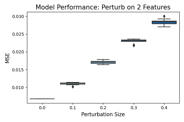
In summary, these plots can be used to assess model robustness under different input perturbation settings, as illustrated in the examples above. The extent to which a model’s performance drops under input perturbation serves as an indication of its robustness. A robust model will exhibit minimal performance degradation when subjected to perturbations.

6.5.2.2. Robustness on worst test samples

In addition to the robustness test on all test samples, we can also test model robustness on worst-performing test samples. To achieve this, we will identify the top \(30\%\) (alpha=0.3) of test samples with the largest absolute residuals. These samples are considered the worst-performing because they have the highest discrepancies between the predicted values and the actual values. Next, we will apply the perturbations to these samples. The perturbation method and perturbation step will remain the same as previously discussed.

exp.model_diagnose(model="FIGS", show="robustness_perf_worst", perturb_features=None,
                  perturb_method="raw", metric="MSE", perturb_size=0.1, alpha=0.3, figsize=(6, 4))

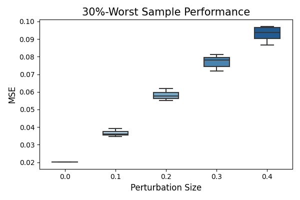
The x-axis shows the noise level (perturbation size), and the y-axis is the model performance (MSE). Under perturbation, we observe that the worst test sample performance is much worse than that of the full test sample. The drop in model performance also increases with the increase in noise level. This plot tells us how poorly the model may perform under the input perturbation and worst cases.

6.5.3. Examples

Example 1: BikeSharing

The first example below demonstrates how to use PiML with its high-code APIs for developing machine learning models for the BikeSharing data from the UCI repository, which consists of 17,389 samples of hourly counts of rental bikes in Capital bikeshare system; see details. The response cnt (hourly bike rental counts) is continuous and it is a regression problem.

• Robustness: Regression

Examples 2: Taiwan Credit

The second example below demonstrates how to use PiML’s high-code APIs for the TaiwanCredit dataset from the UCI repository. This dataset comprises the credit card details of 30,000 clients in Taiwan from April 2005 to September 2005, and more information can be found on the TaiwanCreditData website. The data can be loaded directly into PiML, although it requires some preprocessing. The FlagDefault variable serves as the response for this classification problem.

• Robustness: Classification